Authors: Alex Heaton, Yulia Alexandr, and Sascha Timme
Consider the following problem: Bob has three biased coins. He tosses the first one. If it's heads he chooses the biased coin in his left pocket, and if it's tails he chooses the biased coin in his right pocket. Bob then flips that coin 5 times. We consider those last 5 flips as the experiment. Therefore there are 6 possible outcomes: 0 heads, 1 head, 2 heads, 3 heads, 4 heads, or 5 heads. Can we discover the biases $b_1,b_2,b_3$ of the three coins if we make Bob repeat the entire thing many, many times? Mathematically, we have a 3-dimensional statistical model living inside the 5-dimensional simplex (since probabilities sum to 1).
$$\Delta_5 = \left\{ (p_0,p_1,p_2,p_3,p_4,p_5) \in \mathbb{R}^6 : p_i > 0, \sum p_i = 1 \right\}$$
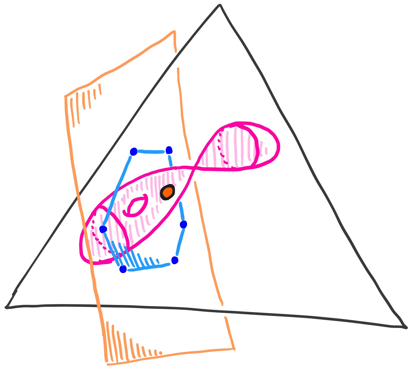
We draw a cartoon of the situation, and explain it below.
In general, you may have a statistical model $\mathcal{M}$ which lives in some probability simplex like $\Delta_5$. Your model may be described by some parameters $\Theta$, like biases of coins. Suppose you want to estimate these parameters, which are unknown to you. You perform experiments and the results produce empirical data $u \in \Delta_5$, which is some point in your simplex. For our example, this data point $(u_0,u_1,u_2,u_3,u_4,u_5)$ could be $(\frac{0}{27},\frac{1}{27},\frac{3}{27},\frac{11}{27},\frac{7}{27},\frac{5}{27})$, where the $\frac{11}{27}$ means Bob got 3 heads in exactly 11 of the 27 experiments he performed. An interesting optimization problem arises naturally: find the point $p$ in your model $\mathcal{M}$ which maximizes the likelihood of your empirical data $u$.
This problem can be solved via Lagrange multipliers. But we are interested in flipping it around. If first we pick our favorite point $p_{fav}$ on the model, then we can ask,
What are all possible empirical data points $u\in\Delta_5$ whose likelihood is maximized by our point $p_{\text{fav}}$?
Say our favorite point is the one pictured in orange, which arises by setting the biases of the coins to $b_1 = \frac{7}{11} $, $b_2 = \frac{3}{5} $, $b_3 = \frac{3}{7}$.
Explicitly this point in our model $\mathcal{M}$ is
$$ p_{\text{fav}} = \Big(\frac{518}{9375}, \frac{124}{625}, \frac{192}{625}, \frac{168}{625}, \frac{86}{625}, \frac{307}{9375}\Big). $$
Choosing this point $p_{\text{fav}}$ defines a 2-dimensional *log-normal space* which is orthogonal to our 3-dimensional model inside the 5-dimensional simplex, in the sense of the log-likelihood function coming from *maximum likelihood estimation* (MLE). This is the orange plane in our cartoon above. The log-likelihood function assigns a (negative) number to every point $p$ in our model, giving the log-likelihood that our data $u$ was produced from the underlying probability distribution given at $p$. We can write this $l_u(p)$.
$$ l_u(p) = \sum_i u_i \text{ log}(p_i) $$
Whichever data points are mapped to our $ p_{\text{fav}} $, surely they live in this log-normal space. In other words, if a data point $u$ is not in the log-normal space to our point $ p_{\text{fav}} $, then $u$ will be closer (in the sense of log-likelihood) to some other point in our model. The question is, which data points $u$ inside the 2-dimensional log-normal space have maximum likelihood estimate $p_{\text{fav}}$?
In fact, we can narrow it down further. Since the simplex consists of points whose coordinates are all positive, our 2-dimensional log-normal space intersects the simplex in a convex polygon, in this case, a hexagon. In fact, for our model, and choice of point $p_{\text{fav}}$, this hexagon is the (2-dimensional) convex hull of the following six vertices:
$$ \begin{array}{rl} &\left(0, \frac{651}{1625}, 0, \frac{30569}{58500}, \frac{43}{2250}, \frac{3377}{58500}\right) \\[1em] & \left(0, \frac{124}{375}, \frac{88}{375}, \frac{77}{375}, \frac{86}{375}, 0\right) \\[1em] &\left(\frac{8288}{76875}, 0, \frac{3176}{5125}, 0, \frac{1376}{5125}, \frac{307}{76875}\right) \\[1em] &\left(\frac{259}{1875}, 0, \frac{52}{125}, \frac{91}{250}, 0, \frac{307}{3750}\right) \\[1em] &\left(\frac{518}{76875}, \frac{1984}{5125}, 0, \frac{2779}{5125}, 0, \frac{4912}{76875}\right) \\[1em] &\left(\frac{2849}{29250}, \frac{31}{1125}, \frac{8734}{14625}, 0, \frac{903}{3250}, 0\right) \end{array} $$
Since we only consider data points $u$ which live in the simplex (because probabilities sum to 1), our question becomes: *which data points $u$ inside the hexagon (which lives inside our log-normal space) have maximum likelihood estimate $p_{\text{fav}}$?*
If we think of maximum likelihood estimation as a map
$$ \phi_{\text{MLE}}: \Delta_5 \longrightarrow \mathcal{M} $$
which sends data points $u$ to their maximum likelihood estimate among the points of our statistical model $\mathcal{M}$, then we are asking for the fibers of this map. For our point $p_{\text{fav}}$, the fiber lives inside the hexagon, which is the 2-dimensional log-normal space to $p_{\text{fav}}$ intersected with the simplex $\Delta_5$. The goal of this example is to use HomotopyContinuation.jl to gain an understanding of what this fiber looks like. The end result will be:
How do we obtain this picture?
From 225 equations to 60000 green and red dots
One can verify that our statistical model is defined by the following five algebraic equations:
$$ \small \begin{array}{rl} f_0 &= p_0+p_1+p_2+p_3+p_4+p_5-1 \\ f_1 &= 20p_0p_2p_4-10p_0p_3^2-8p_1^2p_4+4p_1p_2p_3-p_2^3\\ f_2 &= 100p_0p_2p_5-20p_0p_3p_4-40p_1^2p_5+4p_1p_2p_4+2p_1p_3^2-p_2^2p_3\\ f_3 &= 100p_0p_3p_5-40p_0p_4^2-20p_1p_2p_5+4p_1p_3p_4+2p_2^2p_4-p_2p_3^2\\ f_4 &= 20p_1p_3p_5-8p_1p_4^2-10p_2^2p_5+4p_2p_3p_4-p_3^3 \end{array} $$
We would like to maximize the log-likelihood function at each given point $u$ inside the hexagon and see whether the global maximum happens to be the point $p_{\text{fav}}$. Therefore we consider the gradient of our *objective function*, the log-likelihood function $l_u$, which is given by the following vector each of whose components is a rational function:
$$ \left( \frac{u_0}{p_0}, \frac{u_1}{p_1}, \frac{u_2}{p_2}, \frac{u_3}{p_3}, \frac{u_4}{p_4}, \frac{u_5}{p_5} \right) $$
Using the idea of Lagrange multipliers, we can ask for the gradient of our objective function to be in the span of the gradients of our five equations $f_0, f_1, \dots, f_4$ above, in order to find the critical points. Consider forming a 6$\times$6 matrix from these 6 gradients. Since our model is 3-dimensinal inside the 5-dimensional simplex, the gradients of $f_1$, $f_2$, $f_3$, $f_4$ only contribute rank 2, while the gradient of $f_0$ contributes rank 1. If the gradient of our objective function is in the span of this 3-dimensional space, then our matrix will have exactly rank 3, which is a condition cut out by the 225 $4 \times 4 $ minors of this 6$\times$6 matrix. In conclusion, for a fixed data point $u$, our critical points are the points $p$ which make all 225 minors evaluate to zero. Among these points we will find our global maximum, which might be $p_{fav}$.
$$ \scriptsize \left(\begin{array}{rrrr} 1 & 1 & 1 & … \\ -10 p_3^2 + 20 p_2 p_4 & 4 p_2 p_3 - 16 p_1 p_4 & -3 p_2^2 + 4 p_1 p_3 + 20 p_0 p_4 & …\\ -20 p_3 p_4 + 100 p_2 p_5 & 2 p_3^2 + 4 p_2 p_4 - 80 p_1 p_5 & -2 p_2 p_3 + 4 p_1 p_4 + 100 p_0 p_5 & … \\ -40 p_4^2 + 100 p_3 p_5 & 4 p_3 p_4 - 20 p_2 p_5 & -p_3^2 + 4 p_2 p_4 - 20 p_1 p_5 & … \\ 0 & -8 p_4^2 + 20 p_3 p_5 & 4 p_3 p_4 - 20 p_2 p_5 & …\\ \frac{u_0}{p_0} & \frac{u_1}{p_1} & \frac{u_2}{p_2} & … \end{array}\right. $$
$$ \scriptsize \left.\begin{array}{rrrr} … & 1 & 1 & 1 \\ … & 4 p_1 p_2 - 20 p_0 p_3 & -8 p_1^2 + 20 p_0 p_2 & 0 \\ … & -p_2^2 + 4 p_1 p_3 - 20 p_0 p_4 & 4 p_1 p_2 - 20 p_0 p_3 & -40 p_1^2 + 100 p_0 p_2 \\ … & -2 p_2 p_3 + 4 p_1 p_4 + 100 p_0 p_5 & 2 p_2^2 + 4 p_1 p_3 - 80 p_0 p_4 & -20 p_1 p_2 + 100 p_0 p_3 \\ … & -3 p_3^2 + 4 p_2 p_4 + 20 p_1 p_5 & 4 p_2 p_3 - 16 p_1 p_4 & -10 p_2^2 + 20 p_1 p_3 \\ … & \frac{u_3}{p_3} & \frac{u_4}{p_4} & \frac{u_5}{p_5} \end{array}\right) $$
On the other hand, if we fix our point $p = p_{\text{fav}}$, the $u$ variables only appear linearly in the 4$\times$4 minors of this matrix, since $u$ only appears in the last row. Thus we have linear equations which cut out our 2-dimensional log-normal space of $u$'s at the point $p_{\text{fav}}$. It is inside this space, which forms a hexagon when intersected with the positive orthant, where we will look for our fiber.
The next step is to sample 60000 points $u_i$ from within the hexagon, which lives on our 2-dimensional log-normal plane. We will compute the point which maximizes log-likelihood for each of these points, and color them green if we find $p_{\text{fav}}$, and color them red otherwise. There are many ways to choose these 60000 points. We allowed a computer to generate `random’ barycentric linear combinations of the vertices of the hexagon. Now we have 60000 points $u_i$. For each point, we will solve an optimization problem, finding the point $p_{\text{mle}} \in \mathcal{M}$ in our model which maximizes the log-likelihood function for that fixed $u_i$. If that special point $p_{\text{mle}}$ is our favorite point $p_{\text{mle}} = p_{\text{fav}}$, then we color that point green. If that special point is some other point in our model, $p_{\text{mle}} \neq p_{\text{fav}}$, then we color that point red. In this way, our 60000 points start filling up the hexagon with the colors green and red. The green points will form a region that is a numerical approximation to our fiber, called the Logarithmic Voronoi cell for the point $p_{\text{fav}}$.
Code and random matrix multiplication
How do we set this up in Julia using HomotopyContinuation.jl?
using HomotopyContinuation, DynamicPolynomials, LinearAlgebra
p = @polyvar p0 p1 p2 p3 p4 p5
u = @polyvar u0 u1 u2 u3 u4 u5

f₀ = p0+p1+p2+p3+p4+p5-1
f₁ = 20*p0*p2*p4-10*p0*p3^2-8*p1^2*p4+4*p1*p2*p3-p2^3
f₂ = 100*p0*p2*p5-20*p0*p3*p4-40*p1^2*p5+4*p1*p2*p4+2*p1*p3^2-p2^2*p3
f₃ = 100*p0*p3*p5-40*p0*p4^2-20*p1*p2*p5+4*p1*p3*p4+2*p2^2*p4-p2*p3^2
f₄ = 20*p1*p3*p5-8*p1*p4^2-10*p2^2*p5+4*p2*p3*p4-p3^3
F = [f₀, f₁, f₂, f₃, f₄]
At this point we could try and set up the 6$\times$6 matrix referenced earlier, take all 225 of its minors, and ask HomotopyContinuation.jl to find solutions. However, there may be a more numerically stable way. We describe this method now.
Arrange our polynomial equations $f_0,f_1,f_2,f_3,f_4$ in a vector called $F$. Consider forming the 6$\times$5 matrix $DF$ whose columns are the gradients $\nabla f_i$. As discussed above, we know the dimensions and codimensions, and so we expect that at points $p$ we are interested in, the column space of this matrix will be 3-dimensional, despite its having 5 columns. If we multiply by a random 5x3 matrix $A$, we expect the resulting 6$\times$3 matrix $DF \cdot A$ to span the same column space as $DF$. This random matrix multiplication accomplishes a dimension reduction. Now, if we add a 4th column $u/v$, by which we mean
$$ \left( \frac{u_0}{p_0}, \frac{u_1}{p_1}, \frac{u_2}{p_2}, \frac{u_3}{p_3}, \frac{u_4}{p_4}, \frac{u_5}{p_5} \right)^T, $$
we can clear denominators by multiplying on the left by a diagonal matrix $diag(p_i)$. Introducing new variables, called Lagrange multipliers $\lambda_1, \lambda_2, \lambda_3$, we can require that some linear combination of the first 3 columns is equal to the last column. This gives 6 equations, one for each of the 6 rows of the matrix equation
$$ diag(p_i) \cdot \bigg[DF \cdot A | u/v \bigg] \begin{bmatrix} \lambda_1 \ \lambda_2 \ \lambda_3 \ -1 \end{bmatrix} = 0 $$
In addition to these 6 equations, we include our original 5 equations $f_0,f_1,f_2,f_3,f_4$, which we arrange in a vector $F$ in the code below. In total, we now have 11 equations in the 9 variables, six variables $p_i$ and three variables $\lambda_i$ (rather than 225 equations in 6 variables).
@polyvar la[1:3]
A = randn(ComplexF64, 3, 5)
D_AF = differentiate(A * F, p)
G = [(p .* D_AF') * la .- u; F];
This is a much nicer system of polynomial equations. Now, we could start with a randomly generated point $u_{start}$, substitute, and ask HomotopyContinuation to solve the system for us. We call the resulting solutions starting solutions, because we will use these solutions, obtained via an expensive and long calculation, to more quickly track solutions for the 60000 points $u_i$ that we generated from our hexagon. For more information on this process take a look at our guide An introduction to the numerical solution of polynomial systems.
Now, a naive solve(G) reports that we have to track $110592$ paths. However, by a result in [HKS2005], the maximum likelihood degree of our problem is exactly 39. The ML degree of a statistical model is the number of complex solutions to the system of equations which finds critical points of the log-likelihood function on the model. This means that for generic data $(u_0, u_1,u_2,u_3,u_4,u_5)$ we should find exactly 39 points $p$ on our model which are critical points of the log-likelihood function $l_{u}(p)$. Among these 39 critical points, one of them maximizes the log-likelihood. That critical point is the maximum likelihood estimate on our model which best explains the data $(u_0,u_1,u_2,u_3,u_4,u_5)$.
We could use the solve(G) command to obtain a result in a couple minutes but this approach does not scale for larger systems.
Using monodromy
Instead, we use monodromy. We know that $p_{\text{fav}}$ is a point on our statistical model, so we use it to find just one solution to our system of equations $G$. We pick a random linear combination $\lambda_0$ of the columns, and then solve for what point $u_0$ will give us our $p_{\text{fav}}$.
pfav =  [518/9375, 124/625, 192/625, 168/625, 86/625, 307/9375];
la₀ = randn(ComplexF64, 3)
u₀ = [g_i( p=> pfav) for g_i in (p .* D_AF')] * la₀
We can check that indeed this is a solution.
norm([gᵢ(p => pfav, u => u₀, la => la₀) for gᵢ in G])
which outputs 1.1653e-16. Now we have one legitimate solution to our system of equations $G$. Using monodromy, we can stably and successfully find the other 38. The idea is to perturb our system of equations around a loop, tracking our one legitimate solution along the way. Our system of equations is parametrized by which data point $u_i$ in the simplex we choose. For the parameter $u_0$ above, we know one solution. So we take it for a walk around a loop. When we have returned to our original system of equations (after traversing a loop in parameter space) our original solution will most likely not return to itself, but have moved to another one of the 39 solutions! Now we have two legitimate solutions. We can perturb in another loop, and most likely find 2 new solutions upon our return home. Now we have 4 legitimate solutions. Repeating this process, we are likely to discover all 39 solutions!
In HomotopyContinuation.jl this is very easy to accomplish.
res_generic = monodromy_solve(G, [pfav; la₀], u₀; parameters=[u...], target_solutions_count=39)
which produces the output
Solutions found: 39 	 Time: 0:00:00
MonodromyResult
==================================
• 39 solutions (0 real)
• return code -> success
• 576 tracked paths
• seed -> 153568
With our 39 legitimate starting solutions in hand, we can start to pick our 60000 points, and track solutions, solving the optimization problem for each of them. First, we create our hexagon.
vertices = [
    [0, 651/1625, 0, 30569/58500, 43/2250, 3377/58500],
    [0, 124/375, 88/375, 77/375, 86/375, 0],
    [8288/76875, 0, 3176/5125, 0, 1376/5125, 307/76875],
    [259/1875, 0, 52/125, 91/250, 0, 307/3750],
    [518/76875, 1984/5125, 0, 2779/5125, 0, 4912/76875],
    [2849/29250, 31/1125, 8734/14625, 0, 903/3250, 0]];
rank(hcat(vertices[2:end]...) .- vertices[1])
Our 6 vertices are quite special, since they lie in 2-dimensional affine plane, as the preceding code will discover by outputting a rank of $2$. Below, we translate our polygon so the first of its vertices is at the origin, and use a $QR$ decomposition to find an orthogonal basis for the 2-dimensional plane they span. We write our polygon vertices in terms of this new basis, which means each vertex is encoded by only 2 numbers, not 6, and thus we can plot them.
P = vertices .- Ref(vertices[1])
B = qr(hcat(P...), Val(true)).Q[:,1:2]
coords = Ref(B) .\ P
using Polyhedra, Plots
hexagon = polyhedron(vrep(coords))
plot(hexagon)
Using rejection sampling, we can choose 60000 points inside our hexagon. First we try just 1000 points, to make sure it works.
sampler = let
    poly = hexagon
    # sample from box
    x_min, x_max = extrema(first.(coords))
    y_min, y_max = extrema(last.(coords))
    () -> begin
        while true
            x = rand()*(x_max-x_min) + x_min
            y = rand()*(y_max-y_min) + y_min
            if [x,y] in poly
                return [x,y]
            end
        end
    end
end

test_sample = [sampler() for _ in 1:1000]
plot(hexagon; fill=:transparent)
scatter!(first.(test_sample), last.(test_sample), color=:indianred, markersize=2.5, markerstrokewidth=0)
We are ready to compute. In the following code we sample 60000 points from inside the hexagon, and then track our 39 legitimate starting solutions towards 39 solutions corresponding to each choice of $u_i$ of our 60000 samples. Again, the idea is that we know 39 legitimate solutions at the parameter $u_0$, since we found these using monodromy, starting from just one legitimate solution. Now we can look at our 60000 other parameter points $u_i$ in the hexagon and perturb our system of equations at $u_0$, along with all 39 legitimate solutions, and track them along the way. In this way we can find the 39 solutions for each sample point in the hexagon. We look at all 39 and find which of them maximizes log-likelihood. If it was our favorite point $p_{fav}$, we color that point $u_i$ green. If not, we color that $u_i$ red (or really pink because the plot looked better).
sample_coords = [sampler() for _ in 1:60000]
sample_points = [vertices[1] +  B * v for v in sample_coords];

c₀ = B \ (pfav - vertices[1])

function distance(result, p)
    argmax = nothing
    max_mle = -Inf
    for r in result
        x = r.solution
        is_real_solution = all(i -> abs(imag(x[i])) < 1e-8, 1:6)
        is_real_solution || continue

        pos_solution = all(i -> real(x[i]) >= -1e-8, 1:6)
        pos_solution || continue

        mle = sum(i -> p[i]*log(real(x[i])), 1:6)
        if mle > max_mle
            max_mle = mle
            argmax = [real(x[i]) for i in 1:6]
        end
    end

    norm(pfav - argmax)
end

S = solutions(res_generic)
distances = solve(
    G,
    S;
    parameters = [u...],
    start_parameters = u₀,
    target_parameters = sample_points,
    transform_parameters = distance
)

green = sample_coords[distances .< 1e-8]

plot(hexagon; fill=:transparent)
scatter!(first.(sample_coords), last.(sample_coords), color=:pink, markersize=0.8, markerstrokewidth=0)
scatter!(first.(green), last.(green), color=:green, markersize=1.0, markerstrokewidth=0)
scatter!(c₀[1:1], c₀[2:2], color=:yellow, markersize=5, markerstrokewidth=0)
For more on using monodromy to solve polynomial systems, we recommend the monodromy guide. But finally, the result: Our logarithmic Voronoi cell appears in green, the fibre of $\phi_{MLE}$ above our favorite point $p_{fav}$.
@Misc{ logarithmic-voronoi2026 ,
    author =  { Yulia Alexandr, Alex Heaton, and Sascha Timme },
    title = { Computing a logarithmic Voronoi cell },
    howpublished = { \url{ https://www.JuliaHomotopyContinuation.org/examples/logarithmic-voronoi/ } },
    note = { Accessed: February 5, 2026 }
}