A first example
We are interested in the numerical solution of systems of polynomial equations like $$\begin{array}{rl} -x^5y &= (x^4 + y^4 - 1)(x^2 + y^2 - 2) \\ \frac12 &= x^2+2xy^2 - 2y^2 . \end{array}$$
Equivalently, we can see the solutions of this system of equations as the common zero set $V(f_1,f_2)$ of the polynomials $$ f_1(x,y) = (x^4 + y^4 - 1)(x^2 + y^2 - 2) + x^5y \quad \text{ and } \quad f_2(x,y) = x^2+2xy^2 - 2y^2 - \frac12 . $$ The common zero set $V(f_1,f_2)$ is also called a variety.
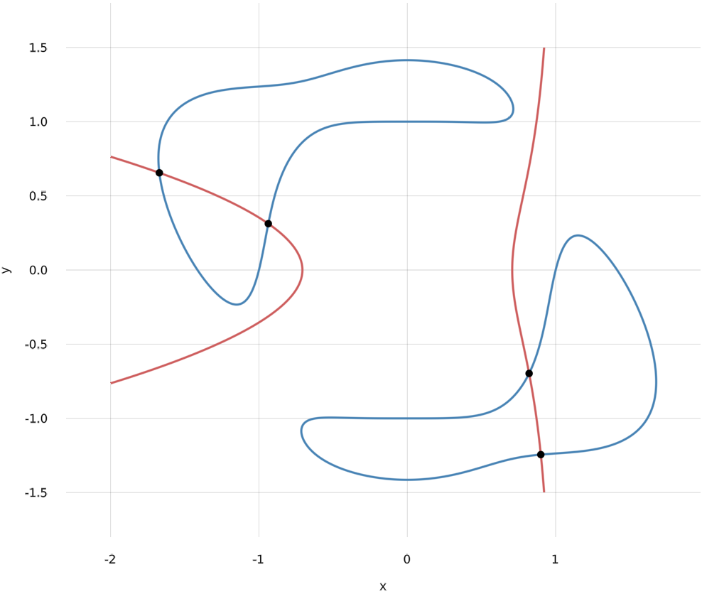
From the figure we can see that $f_1$ and $f_2$ have 4 common zeros. Using HomotopyContinuation.jl we can compute them.
# load the package
using HomotopyContinuation
# declare variables x and y
@var x y
# define the polynomials
f₁ = (x^4 + y^4 - 1) * (x^2 + y^2 - 2) + x^5 * y
f₂ = x^2+2x*y^2 - 2y^2 - 1/2
F = System([f₁, f₂])
result = solve(F)
Result with 18 solutions
========================
• 18 paths tracked
• 18 non-singular solutions (4 real)
• random seed: 0x6baaff3a
• start_system: :polyhedral
Now, the result reports that we found 18 solutions and 4 real solutions. Why do we have 14 solutions more than expected? The reason is that we do not compute the common zero set of $f_1$ and $f_2$ over the real numbers, but over the complex numbers. Although there are usually more complex solutions than real solutions, this makes the problem of computing all real solutions much easier.
The shortest path between two truths in the real domain passes through the complex domain. – J. Hadamard
Since we (for now) only care about the real solutions, we extract them from the result
real_solutions(result)
4-element Vector{Vector{Float64}}:
 [-1.67142, 0.655205]
 [-0.936898, 0.312284]
 [0.820979, -0.697133]
 [0.899918, -1.24418]
The result contains some additional informations about the different solutions.
Let's take a look at the first real solution:
results(result; only_real=true)[1]
   PathResult:
    • return_code → :success
    • solution → ComplexF64[-0.9368979667963298 + 2.938735877055719e-39im, 0.31228408173860095 - 4.70197740328915e-38im]
    • accuracy → 3.4595e-16
    • residual → 6.6613e-16
    • condition_jacobian → 5.5554
    • steps → 50 / 0
    • extended_precision → false
    • path_number → 2
The meaning of those entries is as follows:
return_code → :successmeans that the computation was successful.solutionis the solution that was computed.accuracyis an approximation of $\Vert x-x^* \Vert / \Vert x^* \Vert$ where $x$ is the computed solution and $x^* $ is the true solution.residualis the value of the infinity norm of $f(x)$, where $x$ is the computed solution.condition_jacobianis the condition number of the Jacobian of $f$ at the solution. A large value indicates that this solution is close to being singular.stepsis the number of accepted / rejected steps during the tracking.extended_precisionistrueif it was necessary to use extended precision.path_numberthe number of the path which resulted in this solution.
This is already everything you need to know for solving simple polynomial systems! But in order to solve more challenging systems it is helpful to understand the basics about the techniques used in solve. There are many more advanced features in HomotopyContinuation.jl to help you with solving your particular polynomial system.
Homotopy continuation methods
HomotopyContinuation.jl uses homotopy continuation methods to compute the zero set of polynomial systems (hence the name). The basic idea is as follows:
Suppose that $$F(\mathbf{x})= F(x_1,\ldots,x_n) = \begin{bmatrix} f_1(x_1,\ldots,x_n) \\ \vdots \\ f_m(x_1,\ldots,x_n) \end{bmatrix}$$ is the polynomial system you want to compute the zero set of. Now assume that we have another system $$G(\mathbf{x}) = G(x_1,\ldots,x_n) = \begin{bmatrix} g_1(x_1,\ldots,x_n) \\ \vdots \\ g_m(x_1,\ldots,x_n) \end{bmatrix}$$ where we already know the solutions of and we also know that $G$ has at least as many solutions as $F$.
Furthermore, let's assume that we know how to construct a homotopy $H(\mathbf{x},t)$ such that
- $H(x,1) = G(x)$
- $H(x,0) = F(x)$
- for all $t \in (0,1]$ the polynomial system $H(x,t)$ (in the variables $x_1,\ldots, x_n$) has the same number of isolated zeros.
These are a lof of assumptions but we will see that we always can find $G$ and $H$ which satisfy these conditions.
Tracking solution paths
Now let $y$ be one of the solutions of $G$ resp. a solution of $H$ at $t=1$ and let $x(t)$ be the solution path implicitly defined by the conditions $$H(x(t),t)=0 \quad \text{ and } \quad x(1) = y$$ for $t \in [0,1]$.
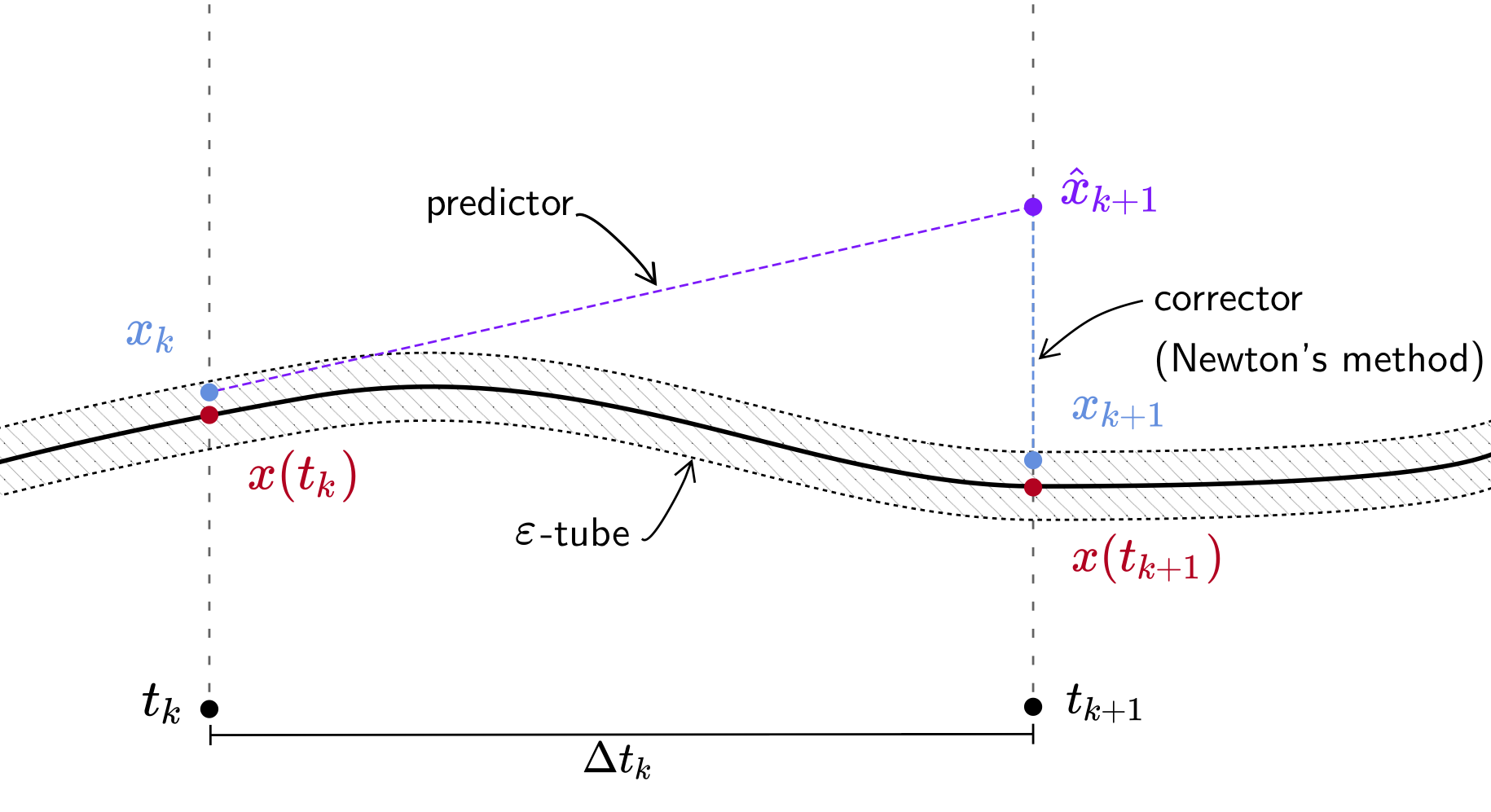
If we now differentiate $H(x(t),t)$ with respect to $t$ we see that the path $x(t)$ is governed by an ordinary differential equation (ODE)! Therefore, we can follow the solution path from $t=1$ to $t=0$ by any numerical method solving ODEs. Every solution $x(t_k)$ at time $t_k$ is a zero of the polynomial system $H(x, t_k)$, and so using Newton's method corrects an approximated solution $x_k \approx x(t_k)$ to an accurate one! We say that we follow the solution path by a predictor-corrector method.
In the following, a path will always mean a solution path in the above sense.
Constructing start systems and homotopies
Homotopy continuation methods work by constructing a suitable start system resp. homotopy. For a given polynomial system there are infinitely many possible start systems and homotopies. We say that a homotopy is optimal if $H(x,1)$ has the same number of solutions as $F(x)=H(x,0)$ since we then only need to track the minimal number of paths possible to still get all solutions of $F(x)$. But constructing optimal homotopies is in general so far not possible. We don't even know an efficient method to compute the number of solutions of $F(x)$. Intersection theory (a part of algebraic geometry) allows to compute this in theory, but proving the number of solutions even for one particular polynomial system is usually worth a research paper.
Instead of aiming at optimal homotopies, we consider polynomial systems as part of a family of polynomial system where we know (or can construct) an optimal homotopy $H(x,t)$ for almost all members of this family. A theorem in algebraic geometry says that the number of solutions of our particular system is always bounded by the number of solutions of the start system $H(x,1)$. The most simple example of this is the total degree homotopy:
Take our initial example $$ f_1(x,y) = (x^4 + y^4 - 1)(x^2 + y^2 - 2) + x^5y \quad \text{ and } \quad f_2(x,y) = x^2+2xy^2 - 2y^2 - \frac12 .$$ The polynomial $f_1$ has degree $6$ and the polynomial $f_2$ has degree 3. Now Bezout's theorem tells us that such a polynomial system has at most $6 \cdot 3=18$ isolated solutions. We then can construct the polynomial system $$g(x,y) = \begin{bmatrix} x^6 - 1 \\ y^3 - 1\end{bmatrix}$$ which has the $18$ solutions $$\left(e^{i 2\pi\frac{k_1}{6}}, e^{i 2\pi\frac{k_2}{3}}\right)$$ where $k_1 \times k_2 \in {0,1,2,3,4,5} \times {0,1,2}$. Then a good homotopy is $$H(x,t) = \gamma t G(x) + (1-t)F(x)$$ where $\gamma \in \mathbb{C}$ is a random complex number with absolute value one.
This construction easily generalizes to polynomial systems with the $n$ polynomials in $n$ variables.
The resulting homotopy is called the total degree homotopy. For a total degree homotopy you have to set the start_system=:total_degree argument.
If we have the system $f=(f_1,\ldots, f_m)$ with degrees $d_1,\ldots, d_m$ then $f$ has at most $d_1 \cdot \ldots \cdot d_n$ many isolated solutions.
For square polynomial systems, i.e., systems with the same number of polynomials and variables there are also more advanced start systems and homotopies which take into account some of the structure of the problem. These include:
- Multi-homogeneous homotopies take a degree structure in the variables into account. This works by using a generalization of Bezout's theorem by Shafarevich.
- Polyhedral homotopies take the sparsity of the polynomials into account. To each polynomial system you can associate the mixed volume of the Newton polytopes of the polynomials. The Bernstein–Khovanskii–Kushnirenko theorem tells us that this mixed volume is an upper bound for the number of isolated solutions with non-zero entries.
Both multi-homogeneous and polyhedral homotopies are supported by HomotopyContinuation.jl.
A multi-homogeneous homotopy is constructed if you pass a set of variable_groups to solve and set start_system=:total_degree.
The polyhedral homotopy is currently the default, but can also be explicitly requested by setting the start_system=:polyhedral argument.
Case Study: Optimization
Consider the distance from a point $u \in \mathbb{R}^n$ to the variety $X=V(f_1,\ldots,f_m)$. We want to solve the following optimization problem:
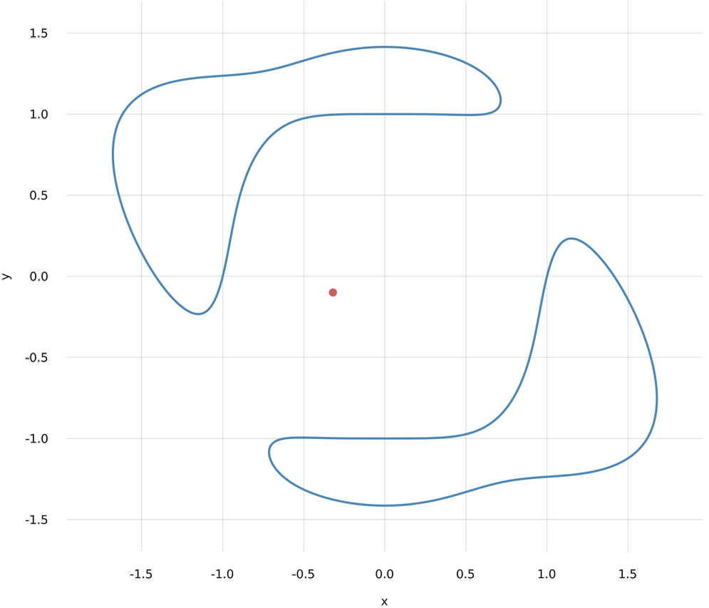
Let us illustrate this with an example. Consider again the polynomial $$f(x,y) = (x^4 + y^4 - 1)(x^2 + y^2 - 2) + x^5y$$ and the point $u_0 = [-0.32, -0.1]$.
We could formulate our problem as the constrained optimization problem
$$\min (x + 0.32)^2 + (y+0.1)^2 \quad \text{ s.t.} \quad f(x,y) = 0 $$
Now this is a non-linear, non-convex minimization problem and therefore it can have multiple local minima as well as local maxima and saddle points. If we approach this problem with a simple gradient descent algorithm starting from a random point we might get as a result a local minimum but we do not know whether this is the global minimum!
In order to make sure that we find the optimal solution we will compute all critical points of this optimization problem. If we count the number of critical points over the complex numbers then this number will almost always be the same. It is called the Euclidean Distance degree of $X=V(f)$.
Solving the critical equations
Let us derive the equations for the critical equations in general in order to apply them afterwards to our example. For a given $u \in \mathbb{R}^n$ and $X=V(f_1,\ldots, f_m)$ we want to solve the problem:
$$\min =||x-u||_2=:d_u(x) \quad \text{subject to} \quad x \in X$$
Considering the geometry of the problem you can see that a point $x^{*} $ is a critical point of the distance function if and only if $x^{*} - u$ is orthogonal to the tangent space of $X$ at $x^{*} $, or formally $$ (x^{*} - u) \perp T_{(x^{*} )}X .$$
Let us assume that $\dim(X)=n-m$ and denote by $J(x)$ the Jacobian of $F=(f_1,\ldots, f_m)$ where the $i$-th row of $J$ consists of the partial derivatives of $f_i$. Then, critical points satisfy the equations $$\begin{array}{rl}x-u &= J(x)^T \lambda \\ F(x) &= 0 \\ \lambda &\in \mathbb{R}^m \end{array}$$
Note: These are the same equations you get from applying Lagrange multipliers to the optimization problem.
Now that we derived the critical equations we can go back to our initial example. Let's start with defining the critical equations in Julia.
# define f
@var x y
f = (x^4 + y^4 - 1) * (x^2 + y^2 - 2) + x^5 * y
# define new variables u₁, u₂ and λ₁
@var u[1:2] λ[1:1]
# define the jacobian of F
J = differentiate([f], [x,y])
# J' defines the transpose of J
C = System([[x,y] - u - J'*λ; f], variables = [x;y;λ], parameters = u)
System of length 3
 3 variables: x, y, λ₁
 2 parameters: u₁, u₂

 -u₁ + x - λ₁*(5*x^4*y + 4*(-2 + x^2 + y^2)*x^3 + 2*(-1 + x^4 + y^4)*x)
 -u₂ + y - (4*(-2 + x^2 + y^2)*y^3 + 2*(-1 + x^4 + y^4)*y + x^5)*λ₁
 x^5*y + (-2 + x^2 + y^2)*(-1 + x^4 + y^4)
We also define the point $u_0 =[-0.32, -0.1]$
u₀ = [-0.32, -0.1]
2-element Vector{Float64}:
 -0.32
 -0.1
Our system $C$ is parametrized by $u$ and we want solve the system for the specific value $u = u_0$.
res = solve(C; target_parameters = u₀)
Result with 36 solutions
========================
• 36 paths tracked
• 36 non-singular solutions (8 real)
• random seed: 0x1556a953
• start_system: :polyhedral
We find that our problem has 36 solutions over the complex numbers, and we can see that there are 8 real solutions.
Let's extract the real points.
# Let's get all real solutions
real_sols = real_solutions(res)
# We have to remove our artifical variable λ₁
ed_points = map(p -> p[1:2], real_sols)
8-element Vector{Vector{Float64}}:
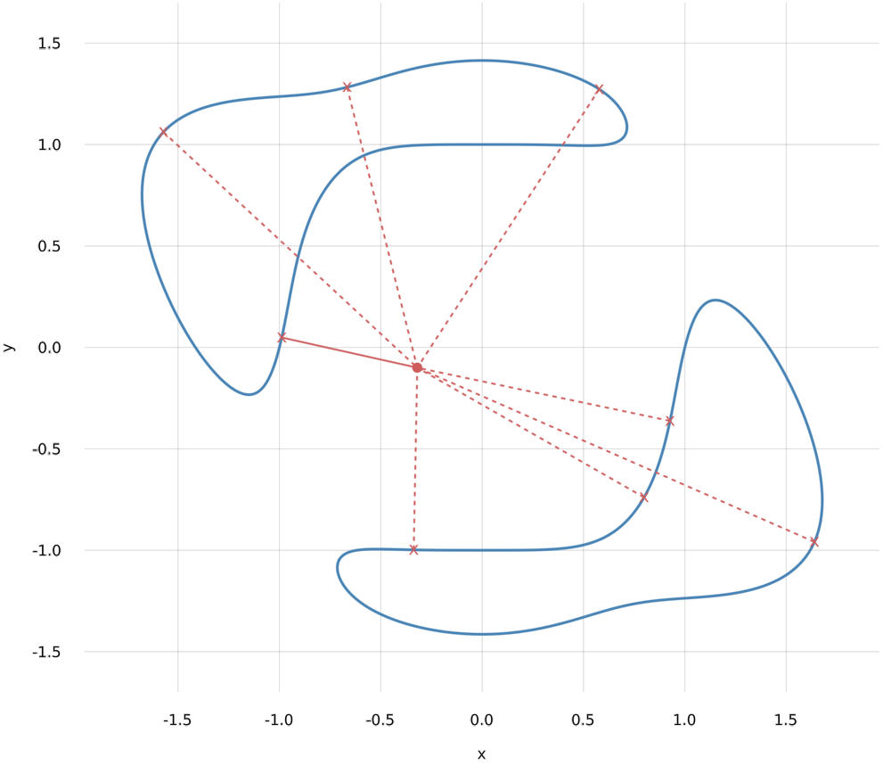
[1.63906, -0.958966]
[0.577412, 1.27259]
[-1.57227, 1.0613]
[0.798736, -0.739109]
[0.926711, -0.362357]
[-0.988532, 0.0487366]
[-0.337537, -0.997977]
[-0.666196, 1.28245]
The optimal solution is found as follows:
using LinearAlgebra

dist, idx = findmin([norm(x - u₀) for x in ed_points])
println("Optimal solution: ", ed_points[idx], " with distance ", dist, " to u₀")
Optimal solution: [-0.988532, 0.0487366] with distance 0.684877 to u₀
Here is a visualization of all (real) critical points:
Computing critical points repeatedly
Now assume you need to solve the optimization problem many times for different values of $u$. We could apply the same computations as above, but note that we needed to track 216 paths in order to find only 36 solutions. Let's make use of the fact that we know that for almost all values of $u$ there are the same number of critical points and that for the other values $u$ the number of isolated solutions can only decrease.
We start with computing all critical points to a random complex value $v \in \mathbb{C}^2$. Let's call the set of 36 critical points $S_v$.
v = randn(ComplexF64, 2)
result_v = solve(C, target_parameters = v)
Result with 36 solutions
========================
• 36 paths tracked
• 36 non-singular solutions (0 real)
• random seed: 0x931f06b2
• start_system: :polyhedral
Remember how we talked above about finding optimal homotopies and how it is hard to do this in general? Well, we just computed an optimal start system and now for a given $u_0$ the homotopy
$$H(x, t) = C_{tv + (1-t)u_0}$$
is an optimal homotopy! $H$ is called a parameter homotopy since we do a homotopy in the parameter space of our (family) of polynomial systems.
This strategy is so essential that we support it out of the box with HomotopyContinuation.jl:
S_v = solutions(result_v)
solve(C, S_v; start_parameters = v, target_parameters = u₀)
Result with 36 solutions
========================
• 36 paths tracked
• 36 non-singular solutions (8 real)
• random seed: 0x9f847e27
We see that only $36$ paths had to be tracked for finding all $36$ critical points of $u_0$.
Note: If the computation of $S_v$ takes some time you should store the solutions (together with $v$!) on your disk. Then you can load them if needed.
Alternative start systems
Sometimes the number of paths to track using a simple solve is very large (or even too large).
Another approach is a technique called monodromy which
uses the fact that our problem has the same number of solutions for almost all values of $u$.
The idea is the following: assume we have parameter $v \in \mathbb{C}^n$ and suppose we know one solution $x_0$ for our problem. We call this a start pair. Now take two other (random) parameter values $v_1, v_2 \in \mathbb{C}^n$ and track the solution $x_0$ with a parameter homotopy from $v$ to $v_1$, then from $v_1$ to $v_2$ and then from $v_2$ back to $v$.
The amazing part is that this loop induces a permutation on all solutions of our system, i.e., even the ones we do not know yet! This means that we can end up with another solution than we started. By doing this process repeatedly we can recover all solutions!
The only condition that we need for this is that the loops we construct contain critical points of the parameter space.
This sound's great so let's try to solve our example using this technique! But how do we obtain a start pair? If you do not provide a start pair, HomotopyContinuation.jl will try to generate a start pair by using Newton's method and random search.
While simple, this is very often successful.
Thus, we can use the monodromy_solve routine to find all solutions often without any additional work.
But for this example, we want to modify the way we construct our loops to ensure that we loop around critical points.
For more compl
parameter_sampler(p) = 10 .* randn(ComplexF64, length(p))
generic_result = monodromy_solve(C; parameter_sampler = parameter_sampler)
MonodromyResult
=========================
• return code → :heuristic_stop
• 36 solutions
• 360 tracked loops
• random seed: 0x590db472
We see that the return code is :heuristic_stop. This comes from the fact that we use a heuristic to determine when we found all solutions and can stop.
The default stopping criterion is to stop after 5 loops without finding any new solutions. We can also set this to another value by
using the max_loops_no_progress flag. Additionally you can set the expected number with the target_solutions_count.
monodromy_solve(C; parameter_sampler = parameter_sampler, max_loops_no_progress=100, target_solutions_count=36)
MonodromyResult
=========================
• return code → :success
• 36 solutions
• 144 tracked loops
• random seed: 0x82046e34
The solutions in the monodromy result can be used for computing the solutions we are interested in.
solve(C, solutions(generic_result); start_parameters=parameters(generic_result), target_parameters=u₀)
Result with 36 solutions
========================
• 36 paths tracked
• 36 non-singular solutions (8 real)
• random seed: 0x6194c170
The monodromy method is very powerful and also has features like the possibility to compute modulo a group action if there is a group acting on the solution set. For more information see our monodromy guide.
More information
If you want to find out more about HomotopyContinuation.jl visit www.JuliaHomotopyContinuation.org. The homepage also contains many examples and guides on how to make the most of numerical homotopy continuation methods. For more informations about the math behind homotopy continuation methods you should check out the book The Numerical Solution of Systems of Polynomials Arising in Engineering and Science by Sommese and Wampler.