Consider a physical system of $N$ particles $q=(q_1,\ldots,q_N)\in M$. In our example we take $M$ to be the space of configurations of cyclohexane. The $q_i$ are then the spacial positions of the six carbon atoms in a cyclohexane molecule. The constraints of this molecule are the following algebraic equations:
$$ M = \{(q_1,\ldots,q_6)\in (\mathbb{R}^3)^6 \mid \Vert q_1-q_2\Vert^2 = \cdots= \Vert q_5-q_6\Vert^2 = \Vert q_6-q_1\Vert^2 = c^2\}, $$
where $c$ is the bond length between two neighboring atoms (the vectors $b_i = q_i - q_{i-1}$ are called bonds). In our example we take $c^2=1$ (unitless).
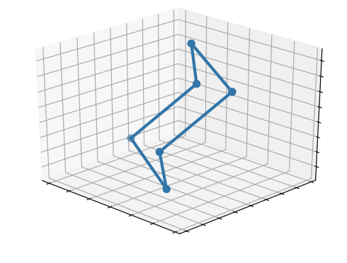
An example of such a configuration is shown in the next picture. It is called the chair.
In the framework of statistical physics, macroscopic quantities of interest are defined as averages over probability measures on all configurations. As the probability measure we take the canonical ensemble. If $E(q)$ denotes the total energy of a configuation $q$, the density of a configuation $q$ in the canonical ensemble is proportional to
$$f(q) = e^{-E(q)}.$$
That is, a configuration is most likely to appear when its energy is minimal. In other words,
configurations that minimize the energy yield macroscopic quantities that we can observe .
In this example we consider as quantitiy the average angle
$$\theta(q)=\frac{1}{6}(\angle(q_6 - q_1, q_2-q_1) + \cdots + \angle(q_5-q_6, q_1-q_6)).$$
between neighboring bonds $q_{i-1} - q_i$ and $q_{i+1} - q_i$, and we compute the macroscopic state of $\theta(q)$. To determine this state we approximate the distribution of $\theta(q)$:
$$\mathrm{Prob} \{\theta(q) = \theta_0\} = \frac{\int_{\theta(q) = \theta_0} f(q) \mathrm{d} q}{K}, $$
where $K=\int_{V} f(q) \mathrm{d} q$ is the normalizing constant.
For comparing the probabilities of different values for $\theta$ it suffices to compute
$$\rho(\theta_0)=\int_{\theta(q) = \theta_0} f(q) \mathrm{d} q.$$
In the following we will approximate this integral using homotopy continuation. At the end of the computation stands the following result summarized in the next plot.
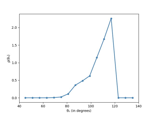
The plot shows a peak at around $\theta = 114^{\circ}$. It is known that the total energy of the cyclohexane system is minimized when all angles between consecutive bonds achieve $110.9^{\circ}$. Our experiment gives a good approximation of the true molecular geometry of cyclohexane. An example where all the angles between consecutive bonds are $110.9^{\circ}$ is shown in the picture above.
Equations for the cyclohexane variety
Due to rotational and translational invariance of the equations we define $q_1$ to be the origin, $q_6=(c,0,0)$ and $q_5$ to be rotated, such that its last entry is equal to zero (like in the cyclooctane example).
We thus have $11$ variables $x(q)=(x_1,\ldots,x_{11})$. Let us implement this in Julia.
using HomotopyContinuation, DynamicPolynomials, LinearAlgebra
c² = 1
N, n = 11, 6

@polyvar x[1:N]
q(x) = [
    zeros(3),
    x[1:3],
    x[4:6],
    x[7:9],
    [x[10]; x[11]; 0.0],
    [√c²; 0; 0]
    ]

F = [(q(x)[i] - q(x)[i+1]) ⋅ (q(x)[i] - q(x)[i+1]) - c² for i in 1:5]
Total energy of a configuration
We model the energy of a molecule using the Lennard Jones interaction potential
$$ V(x,y) = \frac{1}{4}\left(\frac{c}{r}\right)^{12} -\frac{1}{2} \left(\frac{c}{r}\right)^{6}, \text{ where } r=\Vert x-y\Vert. $$
c⁶ = (c²)^3
function V(x,y)
    r⁶ = ((x-y)⋅(x-y))^3
    a = c⁶ / r⁶
    return a^2 / 4 - a / 2
end
The energy function of a configuration $q$ is then.
$$E(q) = \sum_{1\leq i,j\leq N\atop i+2\leq j} V(q_i, q_j).$$
Here is the implementation of $E(q)$ and $f(q)=e^{-E(q)}$.
E(q) = sum(V(q[i], q[j]) for i in 1:5 for j in i+2:6)
f(q) = exp(-E(q))
Integration with homotopy continuation
We approximate
$$\rho(\theta_0) \approx \frac{\mu_1(\theta_0)}{\mu_2(\theta_0)},$$
where
$$ \mu_1(\theta_0) = \int_{\theta(q)>\theta_0 - \Delta\theta\atop \theta(q) < \theta_0 + \Delta\theta} f(q) \mathrm{d} q \text{ and } \mu_2(\theta_0) = \int_{\theta(q)>\theta_0 - \Delta\theta\atop \theta(q) < \theta_0 + \Delta\theta} 1 \mathrm{d} q $$
for some $\Delta \theta >0$. In our experiment we take $\Delta \theta = 3^\circ$ (degrees).
The two integrals are evaluated using the integration guide. Recall from this guide that we have $\mu_1(\theta_0) = \mathbb{E} \overline{f}(A,b),$ where
$$\overline{f}(A,b):= \sum_{q\in M: Ax(q)=b, \atop \theta- \Delta\theta < \theta(q) < \theta + \Delta\theta} \frac{f(q)}{\alpha(q)}\text{ and }\alpha(q) = \frac{\Gamma(\frac{n+1}{2})}{\sqrt{\pi}^{n+1}} \frac{\sqrt{1+\langle x(q), \pi_{x(q)} x(q)\rangle}}{(1+\Vert x(q)\Vert)^{\frac{n+1}{2}}},$$
and where $\pi_x$ is the orthogonal projection onto the normal space $\mathrm{N}_x M$ of $M$ at $x$.
Similarly, we define $\overline{1}(A,b)$ and get $\mu_2(\theta_0)= \mathbb{E} \overline{1}(A,b).$
Let us implement this in Julia. First, we define $\alpha(q)$.
using StaticPolynomials # for fast evaluation of the Jacobian
const SP = StaticPolynomials

F_SP = SP.PolynomialSystem(F)
J(x) = transpose(SP.jacobian(F_SP, x))
function α(x₀)
    J₀ = J(x₀)
    U = Matrix(qr(J₀).Q)
    π_x₀ = U * (transpose(U) * x₀)
    return sqrt(1 + (x₀ ⋅ π_x₀)) /  sqrt(1 + (x₀ ⋅ x₀))^(n+1)
end
We also need a function for the evaluation of $\theta(q)$.
θ(q) = (1/6) * (
    ∠(q[6]-q[1], q[2]-q[1]) +
    ∠(q[1]-q[2], q[3]-q[2]) +
    ∠(q[2]-q[3], q[4]-q[3]) +
    ∠(q[3]-q[4], q[5]-q[4]) +
    ∠(q[4]-q[5], q[6]-q[5]) +
    ∠(q[5]-q[6], q[1]-q[6])
    )

function ∠(b₁, b₂)
  γ = normalize(b₁) ⋅ normalize(b₂)
  if γ > 1
      return 0.0
  elseif γ < -1
      return pi
  else
      return acos(γ)
  end
end
Now we implement $\overline{f}(A,b)$. We estimate the integrals $\mu_1$ and $\mu_2$ separately, and we have to define $\overline{f}(A,b)$ for both integrals separately. To take this into account, we implement the integrand $f$ as an input for f̄. The range of integration θ₀ - Δθ ≦ θ ≦ θ₀ + Δθ is also an input for to f̄.
using SpecialFunctions
const SF = SpecialFunctions
Γ = pi^(n+1) / SF.gamma((n+1)/2)

function f̄(R, θ₀, Δθ, f)
    s = 0.0
    θl, θu = θ₀ - Δθ, θ₀ + Δθ
    if nreal(R) > 0
        for xᵢ in real_solutions(R)
            qᵢ = q(xᵢ)
            if θl < θ(qᵢ) < θu
                s += f(qᵢ) / α(xᵢ)
            end
        end
    end
    Γ .* s
end
Finally, to intersect the cyclohexane variety with linear spaces we create an artificial start system and compute its complex solutions.
@polyvar A[1:n, 1:N] b[1:n]
G = [F; A * x - b]

A₀, b₀ = randn(ComplexF64, n, N), randn(ComplexF64, n)
G₀ = [subs(g, vec(A) => vec(A₀), b => b₀) for g in G]
start_sols = solutions(solve(G₀));
Computing the distribution of $\theta$
Now, we can compute the approximation of $\rho(\theta_0)$. We use $k=10^4$ linear sections and choose values $\frac{\pi}{4}\leq \theta_0\leq \frac{3\pi}{4}$.
First, we compute the empirical distributions for $f̄$ from which we infer $\mu_1$.
k  = 10^4,
Δθ = 3 * (2pi/360)
θs = pi/4 : 2*Δθ : 3pi/4
empirical_distributions_f̄ = map(θs) do θ₀
    S = solve(
        G,
        start_sols;
        parameters = [vec(A); b],
        start_parameters =  [vec(A₀); b₀],
        target_parameters = [randn(n*N + n) for _ in 1:k],
        transform_result = (R,p) -> f̄(R, θ₀, Δθ)
    )
end
Then, we compute the empirical distributions for $\overline{1}$ from which we infer $\mu_2$.
empirical_distributions_const1̄ = map(θs) do θ₀
    S = solve(
        G,
        start_sols;
        parameters = [vec(A); b],
        start_parameters =  [vec(A₀); b₀],
        target_parameters = [randn(n*N + n) for _ in 1:k],
        transform_result = (R,p) -> f̄(R, θ₀, Δθ, qᵢ -> 1.0)
    )
end
Here are the estimates for the distribution of $\theta$:
using  Statistics
μ₁ = mean.(empirical_distributions_f̄)
μ₂ = mean.(empirical_distributions_const1̄)
# such that ρ = μ₁ ./ μ₂
# but  μ₁ ./ μ₂ has NaN entries, because μ₂ has zero entries
# we have to filter out the NaNs
ρ = map(m -> isnan(m) ? 0.0 : m, μ1 ./ μ2)
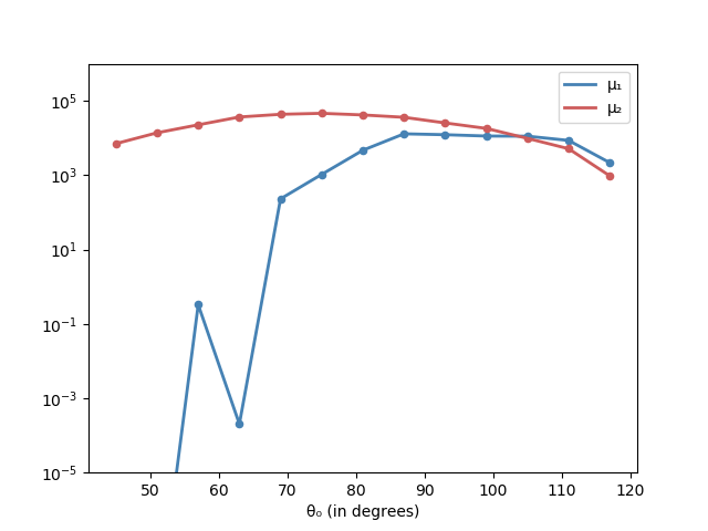
The next plot shows $\mu_1$ and $\mu_2$ in the logarithmic scale:
Rate of convergence
How good is the estimate? The analysis of variance from the the integration guide yields for the empirical mean $\mathrm{E}(f,k) = \frac{1}{k}(\overline{f}(A_1,b_1) + \cdots \overline{f}(A_k,b_k))$:
$$\mathrm{Prob}\{\vert \mathrm{E}(f,k) - \mu_1(\theta_0) \vert \geq \varepsilon \} \leq \frac{\sigma^2}{\varepsilon^2k},$$
where $\sigma^2$ is the variance of $\overline{f}(A,b)$ and similar for $E(1,k)$. From the plot above we can deduce that
ε = 1e2
is a good accuracy for both $\mu_1(\theta_0)$ and $\mu_2(\theta_0)$.
Using the empirical variances to approximate the true variance we get the following:
julia> s²(f̄) = std.(empirical_distributions_f̄)
julia> maximum(s²(f̄) ./ (ε^2 * k))
0.0018945016028972723
and
julia> s²(const1̄) = std.(empirical_distributions_const1̄)
julia> maximum(s²(const1̄) ./ (ε^2 * k))
0.0018301742629020274
That is, the maximum deviation probability is less than $1$% in both cases. We conclude that our approximation of $\rho(\theta) = K\mathrm{Prob}\{\theta(q) = \theta_0\}$ is a good approximation.
Cite this example:
@Misc{ energy-minimization2026 ,
    author =  { Paul Breiding },
    title = { Energy minimization },
    howpublished = { \url{ https://www.JuliaHomotopyContinuation.org/examples/energy-minimization/ } },
    note = { Accessed: February 5, 2026 }
}