Consider the problem of numerically approximating an integral of the form
$$\int_{V} f(x) \mathrm{d}x,$$
where $V\subset \mathbb{R}^N$ is an open submanifold of an algebraic variety and $f:V\to \mathbb{R}$ is a measurable function.
For instance, for $f(x)=1$, this integral gives the volume of $V$. In this example, we want to use homotopy continuation to approximate this integral. We will use the Monte Carlo integration proposed in this article.
Integrating functions with homotopy continuation
Let $n=\mathrm{dim} V$, and let $A\in \mathbb{R}^{n\times N}$ and $b\in \mathbb{R}^n$ be a matrix-vector pair with independent standard Gaussian entries. Then, almost surely, $\{x\in \mathbb{R}^N : Ax=b\}$ is a linear space of dimension $N-n$, which intersects $V$ in finitely many points.
Consider the random variable
$$\overline{f}(A,b):= \sum_{x\in V: Ax=b} \frac{f(x)}{\alpha(x)},$$
where
$$\alpha(x) = \frac{\Gamma(\frac{n+1}{2})}{\sqrt{\pi}^{n+1}} \frac{\sqrt{1+\langle x, \pi_x x\rangle}}{(1+\Vert x\Vert)^{\frac{n+1}{2}}}$$
and where $n=\mathrm{dim}(V)$, and where $\pi_x$ is the orthogonal projection onto the normal space of $V$ at $x$. The main theorem of the article yields
$$\mathbb{E} \overline{f}(A,b) = \int_V f(x) \mathrm{d} x.$$
The empirical mean $\mathrm{E}(f,k) = \frac{1}{k}(\overline{f}(A_1,b_1) + \cdots \overline{f}(A_k,b_k))$ for $k$ sample pairs $(A_1,b_1),\ldots, (A_k,b_k)$ converges to the integral of $f$ over $V$ as $k\to \infty$.
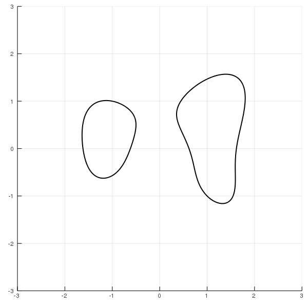
Example: volume of a planar curve
Let us now use the empirical mean of $\overline{f}(A,b)$ for $f(x)=1$ to approximate the volume of the curve $C = \{x^4+y^4-3x^2-xy^2-y+1 = 0\}$. A plot of the curve is shown next.
Let us define the equation for $C$ in Julia.
using HomotopyContinuation, LinearAlgebra, Statistics
@var x[1:2]
F = [x[1]^4+x[2]^4-3x[1]^2-x[1]*x[2]^2-x[2]+1]
We also define $\overline{f}$.
f(x) = 1.0 # so that ∫ f(x) dx gives the volume

using SpecialFunctions
N, n = 2, 1
Γ = SpecialFunctions.gamma((n+1)/2) / sqrt(pi)^(n+1)
J = differentiate(F, x)

#define f̄
function f̄(R)
    if nreal(R) == 0
        return 0.0
    else
        return sum(z -> f(z) / α(z, J), real_solutions(R))
    end
end
function α(z, J)
    Q, R = qr(J(x=>z)')
    NₓM = Q[:, 1:(N - n)] * (Q[:, 1:(N - n)])'
    return sqrt(1 + z⋅(NₓM * z)) / sqrt((1 + z⋅z)^(n+1)) * Γ
end
For computing $f(A,b)$ we have to intersect $V$ with linear spaces. Following this guide we first create a suitable start system by intersecting $V$ with a random complex linear space of dimension $N-n$.
L₀ = rand_subspace(N; dim = N - n)
start = solve(F, target_subspace = L₀)
start_sols = solutions(start)
Now, we track start_sols towards $10^5$ random Gaussian linear spaces.
k = 10^5
#track towards k random linear spaces
empirical_distribution = solve(
    F,
    start_sols;
    start_subspace =  L₀,
    target_subspaces = [rand_subspace(N; dim = N - n, real = true) for _ in 1:k],
    transform_result = (R,p) -> f̄(R)
)
We get the following estimate for the volume:
julia> mean(empirical_distribution)
11.203665864791367
Rate of convergence
Let $\sigma^2$ be the variance of $\overline{f}(A,b)$. By Chebychevs inequality we have the following rate of convergence for the $k$-th empirical mean $\mathrm{E}(f,k) = \frac{1}{k}(\overline{f}(A_1,b_1) + \cdots \overline{f}(A_k,b_k))$:
$$\mathrm{Prob}\{\vert \mathrm{E}(f,k) - \int_V f(x) \mathrm{d} x \vert \geq \varepsilon \} \leq \frac{\sigma^2}{\varepsilon^2k}.$$
The empirical variance of our sample is
julia> s² = std(empirical_distribution)
8.198196919934363
For $\varepsilon = 0.1$ the probability of $\vert \mathrm{E}(1,k) - \mathrm{vol}(V)\vert\geq \varepsilon$ is
julia> ε = 0.1
julia> s² / (ε^2 * k)
0.008198196919934361
Therefore, we can safely conclude that $\mathrm{vol}( C ) \approx 11.2$.
Cite this example:
@Misc{ monte-carlo-integration2026 ,
    author =  { Paul Breiding },
    title = { Monte Carlo integration },
    howpublished = { \url{ https://www.JuliaHomotopyContinuation.org/examples/monte-carlo-integration/ } },
    note = { Accessed: February 5, 2026 }
}