The reach $\tau$ of an embedded manifold $M\subset \mathbb{R}^n$ is an important complexity measure for methods in computational topology, statistics and machine learning. Namely, estimating $M$, or functionals of $M$, requires regularity conditions and a common regularity assumption is that the reach $\tau >0$. The definition of $\tau$ is as follows:
$$\tau = \sup \{t\mid \text{all $x\in\mathbb{R}^n$ with $\mathrm{dist}(x,M)<t$ have a unique nearest point on $M$}\}$$
where the distance measure $\mathrm{dist}$ is the Euclidean distance.
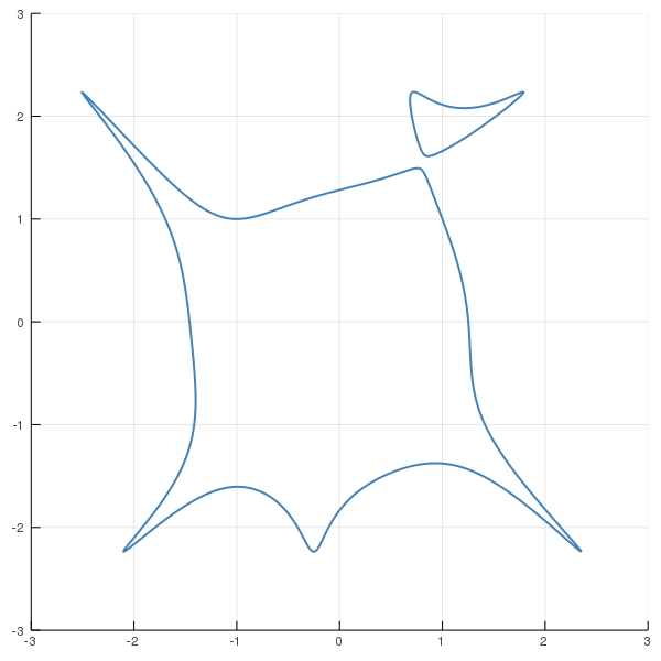
In this example we want to compute the reach of an algebraic manifold; that is, an embedded manifold which is also an algebraic variety. The variety we consider is the plane curve $C$ defined by the equation
$$ f(x,y) = (x^3 - xy^2 + y + 1)^2(x^2+y^2 - 1)+y^2-5 = 0 $$
As pointed out by Aamari et. al. the reach is the determined by the bottlenecks of $C$, which quantify how close $C$ is from being self-intersecting, and the curvature of $C$:
$$\tau = \min\left\{\frac{\rho}{2}, \frac{1}{\sigma}\right\},$$
where $\sigma$ is a the maximal curvature of a geodesic running through $C$ and $\rho$ is the width of the narrowest bottleneck of $C$.
We compute both $\rho$ and $\sigma$. For this, we first define the equation of $C$ in Julia.
using HomotopyContinuation
@polyvar x y
f = (x^3 - x*y^2 + y + 1)^2 * (x^2 + y^2 - 1) + y^2 - 5
Our computation below finds
$$\rho \approx 0.13835 \text{ and }\ \sigma \approx 2097.17$$
and therefore the reach of the curve $C$ is
$$\tau \approx \min\left\{\frac{0.13835}{2}, \frac{1}{2097.167}\right\} \approx 0.000479.$$
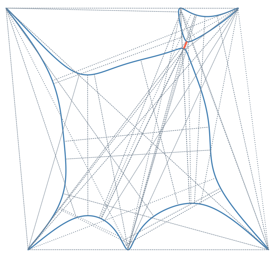
Bottlenecks
Bottlenecks of $C$ are pairs of points $(p,q)\in C\times C$ such that $p-q$ is perpendicular to the tangent space $\mathrm{T}_p C$ and perpendicular to the tangent space $\mathrm{T}_q C$.
Eklund and di Rocco et. al. discuss the algebraic equations of bottlenecks. The equations are
$$f(p) = 0, \quad \det\begin{bmatrix} \nabla_p f & p-q\end{bmatrix} = 0, \quad f(q) = 0 ,\quad \det\begin{bmatrix} \nabla_q f & p-q\end{bmatrix}=0,$$
where $\nabla_p f$ denotes the gradient of $f$ at $p$. The first equation defines $p\in C$ and the second equation defines $p-q \perp \mathrm{T}_p C$. The third equation defines $q\in C$ and the fourth equation defines $p-q \perp \mathrm{T}_q C$.
The width of a bottleneck is $\rho(p,q) = \Vert p-q\Vert_2$. The width of the narrowest bottleneck is the minimum over all $\rho(p,q)$ such that $(p,q)$ satisfies the above equations.
Let us define and solve the equations in Julia:
using LinearAlgebra: det

@polyvar p[1:2] q[1:2] # define variables for the points p and q
f_p = subs(f, [x;y] => p)
f_q = subs(f, [x;y] => q)
∇_p = differentiate(f_p, p)
∇_q = differentiate(f_q, q)
bn_eqs = [f_p; det([∇_p p-q]); f_q; det([∇_q p-q])]

bn_result = solve(bn_eqs, start_system = :polyhedral)
Result{Array{Complex{Float64},1}} with 1858 solutions
=====================================================
• 1726 non-singular solutions (104 real)
• 132 singular solutions (0 real)
• 3600 paths tracked
• random seed: 577138
• multiplicity table of singular solutions:
┌───────┬───────┬────────┬────────────┐
│ mult. │ total │ # real │ # non-real │
├───────┼───────┼────────┼────────────┤
│   1   │  60   │   0    │     60     │
│   2   │  72   │   0    │     72     │
└───────┴───────┴────────┴────────────┘
From bn_result we see that $C$ has $1726$ (complex) bottleneck pairs and of those are
$104$ real. Note that in our formulation we have for each bottleneck pair $(p,q)$
also the pair $(q, p)$ as a solution. Therefore we find that the curve $C$ has $52$ distinct real bottlenecks.
From the real solutions we compute the width of the narrowest bottleneck.
bn_pairs = real_solutions(nonsingular(bn_result))
ρ = map(s -> norm(s[1:2] - s[3:4]), bn_pairs)
ρ_min, ρ_min_ind = findmin(ρ)
(0.13835123592621543, 22)
We see that the narrowest bottleneck of $C$ is of width $\rho \approx 0.13835$.
Finally, we want to plot all bottlenecks. The narrowest bottleneck is highlighted in red.
using Plots, ImplicitPlots

# Show curve
implicit_plot(f; dpi=200, axis=false, grid=false)
# Draw all bottlenecks in gray with dashed lines
for (p₁,p₂,q₁,q₂) in bn_pairs
  plot!([p₁, q₁], [p₂, q₂];
        color = :slategray, grid=false, linestyle=:dot)
end
# Draw narrowest bottleneck in red
narrowest_bn_pair = bn_pairs[ρ_min_ind]
plot!(narrowest_bn_pair[[1,3]], narrowest_bn_pair[[2,4]];
      color = :tomato, grid=false, linewidth = 3)
Maximal curvature
The following formula gives the curvature $\sigma(p)$ at $p\in C = \{f(x,y)=0\}$.
$$\sigma(p) = \frac{h(p)}{g(p)^\frac{3}{2}}$$
where
$$g(p)= \nabla_p f^T\nabla_p f\quad \text{and}\quad h(p) = v(p)^T H(p) v(p),$$
and where $H(p)$ is the Hessian of $f$ at $p$ and $v(p) = \begin{bmatrix} 0 & -1 \\ 1 & 0 \end{bmatrix}\nabla_p f$.
For computing the maximum of $\sigma(p)$ over $C$ we solve the critical equations of $\sigma(p)$.
The critical equations are
$$v(p)^T \nabla_p \sigma=0\quad \text{and}\quad f(p)=0.$$
We use the following code.
∇ = differentiate(f, [x;y]) # the gradient
H = differentiate(∇, [x;y]) # the Hessian

g = ∇ ⋅ ∇
v = [-∇[2]; ∇[1]]
h = v' * H * v
dg = differentiate(g, [x;y])
dh = differentiate(h, [x;y])

∇σ = g .* dh - ((3/2) * h).* dg

F₂ = [v ⋅ ∇σ; f]

curv_result = solve(F₂, start_system = :polyhedral)
Result{Array{Complex{Float64},1}} with 176 solutions
====================================================
• 176 non-singular solutions (24 real)
• 0 singular solutions (0 real)
• 292 paths tracked
• random seed: 140163
From curv_result we see that C has $176$ (complex) points of critical curvature and of those are
$24$ real. From the result we compute the corresponding curvatures and extract the maximum.
curv_pts = real_solutions(nonsingular(curv_result))
σ(s) = h(s) / g(s)^(3/2)
σ_max, σ_max_ind = findmax(σ)
(2097.165767782749, 23)
Therefore, the maximal curvature of a geodesic in $C$ is $\sigma \approx 2097.17$.
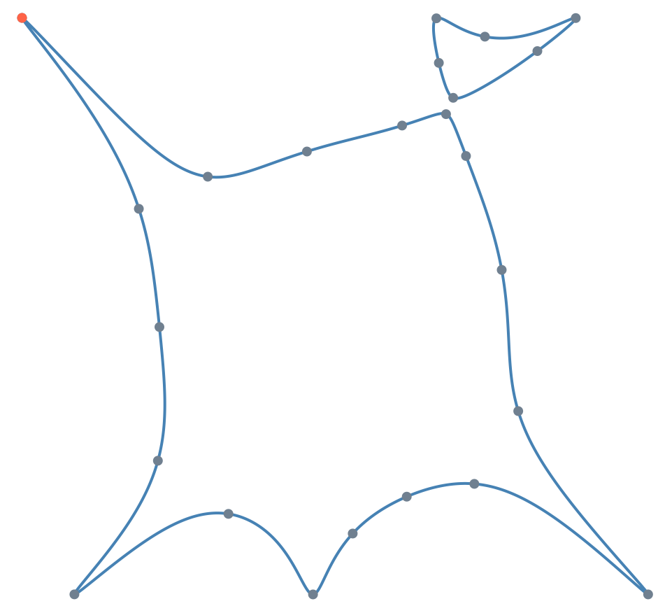
Here is a plot of all critical points in green with the point of maximal curvature in red.
implicit_plot(f; dpi=200, axis=false, grid=false)
scatter!(first.(curv_pts), last.(curv_pts);
         markerstrokewidth=0, markersize=4,
         color=:slategray, grid=false)
# Draw point of maximal curvature
max_curv_pt = R₂[σ_max_ind]
scatter!(max_curv_pt[1:1], max_curv_pt[2:2];
         markerstrokewidth=0, markersize=4,
         color=:tomato, grid=false)
@Misc{ reach-curve2026 ,
    author =  { Paul Breiding and Sascha Timme },
    title = { The reach of a plane curve },
    howpublished = { \url{ https://www.JuliaHomotopyContinuation.org/examples/reach-curve/ } },
    note = { Accessed: February 5, 2026 }
}