This post was worked out in a student seminar that we held at TU Berlin in summer 2019.
We want to reconstruct a three-dimensional object from two-dimensional images. Think of an object, maybe a dinosaur, that is captured by $n$ cameras from different angles. Suppose we have the following information available:
- the configuration of the cameras (in the form of camera matrices);
- sets of 2D points in the $n$ two-dimensional images, where each set corresponds to one 3D point.
(Actually, the second bullet is the more challenging part in reconstructing three-dimensional objects. We assume that this task has already been done.)
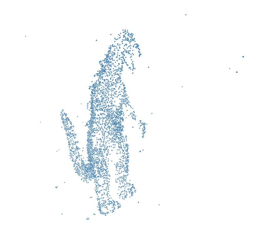
The goal is to compute the following 3D picture
In theory, it suffices to have two matching 2D points and the configuration of the cameras to exactly reconstruct the corresponding 3D point. In practice, there is lens distortion, pixelation, the algorithm matching the 2D points is not working fully precise and so on. This is why we are looking for 3D points that minimize the euclidean distance regarding their 2D image points. We want to solve an optimization problem.
This post is restricted to the case $n=2$, i.e. we want to reconstruct 3D points from images captured by two cameras at a time. We take the dinosaur data set from the Visual Geometry Group Department of Engineering Science at the University of Oxford. This contains a list of 36 cameras as $3\times 4$ matrices and a corresponding list of pictures taken from 4983 world points. (For using the code below one must download the files from these links.)
Let $x\in\mathbb{R}^3$ be a 3D point. Then, taking a picture $u=(u_1,u_2)\in\mathbb{R}^2$ of $x$ is modeled as
$$ \begin{pmatrix} u_1 \\ u_2 \\ 1 \end{pmatrix} = t A \begin{pmatrix}x_1 \\ x_2 \\ x_3 \\ 1\end{pmatrix},$$
where $A\in \mathbb{R}^{3\times 4}$ is the camera matrix and $t \in \mathbb{R}, t \neq 0$, is a scalar. This is called the pinhole camera model. Let us write $y(x)$ for the first two entries of $A \begin{pmatrix} x\\ 1\end{pmatrix}$, and $z(x)$ for the third entry. Then, $u=t y(x)$ and $1 = t z(x)$.
If $p = (p_1, p_2) \in\mathbb{R}^2\times \mathbb{R}^2$ are two input pictures from the data set, we want to solve the following minimization problem:
$$ \underset{(x,t) \in \mathbb{R}^3\times (\mathbb{R}\backslash \{0\})^2}{\operatorname{argmin}} \lVert t_1 y_1(x) - p_1 \rVert^2 + \lVert t_2 y_2(x) - p_2 \rVert^2 $$
$$ \text{s.t. } t_1 z_1(x) = 1 \text{ and } t_2 z_2(x)=1.\quad $$
Implementation with Homotopy Continuation
Now let's solve this optimization problem using homotopy continuation by solving the critical equations. We use the cameras n₁=1 and n₂=2. The camera data
using HomotopyContinuation, LinearAlgebra

# download camera and pictures data and load it
include(download("https://gist.githubusercontent.com/PBrdng/46436855f3755c5a959a7c5d6ba7e32b/raw/5e6be8f4c9673f0dd26010b5e0cefc8e953fc1c0/cameras.jl"))
include(download("https://gist.githubusercontent.com/PBrdng/46436855f3755c5a959a7c5d6ba7e32b/raw/5e6be8f4c9673f0dd26010b5e0cefc8e953fc1c0/pictures.jl"))
n₁, n₂ = 1, 2
camera_numbers = [n₁, n₂]

@var x[1:3]
@var t[1:2]
@var p[1:2,1:2]

y = [cams[i][1:2,:]*[x; 1] for i in camera_numbers]
z = [cams[i][3,:] ⋅ [x; 1] for i in camera_numbers] .* 648
The last multiplication by 648 is because the data is given in pixel units (between 0 and 648). For numerical stability it is better to work with coordinates between 0 and 1. Now, we define the target function.
g = [t[i] .* y[i] - p[:,i] for i in 1:2]
G = sum(gᵢ ⋅ gᵢ for gᵢ in g)
# G is the function that we want to optimize
For G we generate the critical equations F=0 using Lagrange multipliers.
@var λ[1:2] # the Lagrance multipliers
L = G - sum(λ[i] * (t[i] * z[i] - 1) for i in 1:2)
∇L = differentiate(L, [x;t;λ])
F = System(∇L; variables = [x;t;λ], parameters = vec(p))
F is a system of polynomials in the variables x, t and λ and the parameters p. We want to solve this system many times for different parameters. For this, we use the guide on how to track many systems in a loop.
First, we need an initial solution for a random set of parameters.
p₀ = randn(ComplexF64, 4)
start = solutions(solve(F; target_parameters = p₀))
start contains 6 solutions. At the end of this example we discuss that the number of critical points F=0 is indeed 6. Now, we track these 6 solutions towards the photo parameters we are interested in.
#first, we need to preprocess the photo data
photos = [ps[i, [2 * n₁ - 1, 2 * n₁, 2 * n₂ - 1, 2 * n₂]] for i in 1:4983]

# the data from the dataset is incomplete.
# the cameras did not take pictures of all world points.
# if a world point was not captured, the entry in the data set is -1.
filter!(pᵢ -> all(pᵢ .> 0), photos)

# we divide the photo coordinates by 648
# to work with coordinates between 0 and 1
# (as explained above)
map!(pᵢ -> pᵢ./648, photos, photos)

function reconstruction_from_critical_points(R, pᵢ, G)
	r = real_solutions(R)
	N = map(r) do rᵢ
		G([x;t] => rᵢ[1:5], vec(p) => pᵢ)
	end
	i = findmin(N)

	return r[i[2]][1:3]
end


reconstructed_points = solve(
    F,
    start;
    start_parameters =  p₀,
    target_parameters = photos,
    transform_result = (R,pᵢ) -> reconstruction_from_critical_points(R,pᵢ,G)
)
Doing this for several pairs of cameras we get the above picture.
EDdegree of the Multiview variety
The closure (under Zariski topology) of
$$\{(t_1y_1(x), t_2y_2(x))\in \mathbb{R}^2\times \mathbb{R}^2 \mid t_1z_1(x) = t_2z_2(x) = 1, (x,t)\in \mathbb{R}^3 \times (\mathbb{R}\backslash \{0\})^2\}$$
is called (affine) multiview variety for two cameras.
Regarding such an affine multiview variety, the number of (complex) critical points of the squared distance function G is an invariant, which is called the euclidean distance degree (ED degree). Maxim, Rodriguez and Wang proved showed that the EDdegree of the Multiview variety for 2 cameras is 6. We used this information in the code above for verifying that the initial computation for F₀ was correct.
@Misc{ computer-vision2026 ,
    author =  { Paul Breiding, Christoph Schmidt },
    title = { Computer vision },
    howpublished = { \url{ https://www.JuliaHomotopyContinuation.org/examples/computer-vision/ } },
    note = { Accessed: February 5, 2026 }
}