Alt's problem

A classical problem from robotics

8 minute read Published: 28 Oct, 2019

This post currently is only valid for HomotopyContinuation v1

This post was worked out in a student seminar that we held at TU Berlin in summer 2019.

A four bar linkage, also called four bar, is a mechanism of four bars connected in a loop by four joints. One bar is fixed to the ground and on top of the opposing bar sits a triangle called coupler triangle whose apex is called coupler point. In motion this coupler point follows a curve called coupler curve:

The synthesis problem describes the problem of finding all four bars whose coupler curve passes through a given number of precision points. The largest possible number of prescribed precision points is $9$. This problem was first formulated by Alt in 1923 and completely solved by Wampler et al. in 1992 using homotopy continuation.

In case the reader just wants to create videos like the one above, we have created a shortcut:

using Pkg
pkg"add https://github.com/JuliaHomotopyContinuation/FourBarLinkages.jl.git"
using FourBarLinkages

# coupler points in isotropic coordinates
coupler_points = [
    complex(0.8961867,-0.09802917),
    complex(1.2156535, -1.18749100),
    complex(1.5151435, -0.85449808),
    complex(1.6754775,  -0.48768058),
    complex(1.7138690,-0.30099232),
    complex(1.7215236,0.03269953),
    complex(1.6642029, 0.33241088),
    complex(1.4984171, 0.74435576),
    complex(1.3011834,  0.92153806)
]

# compute four bar linkages for the couple points from the stored results
fourbars = four_bars(coupler_points)

# pick a fourbar
F = fourbars[3]
# animate
animate(F, coupler_points)
# create endless loop (interrupt to stop)
animate(F, coupler_points; loop=true)
# save animation and hide axis
animate(F, coupler_points; filename="four-bar.gif", show_axis=true)

In the rest of this example, based on Wampler et. al., we will show how we can implement an adapted algorithm in Julia using HomotopyContinuation.jl.

Constructing the polynomial system

First up we will derive the polynomial system describing the problem.

Instead of looking at the bars as vectors in $\mathbb{R}^2$, we will look at them as vectors in the complex plane.

First we observe the relation of the triangles $ADP$ and $BPC$ from the next picture.

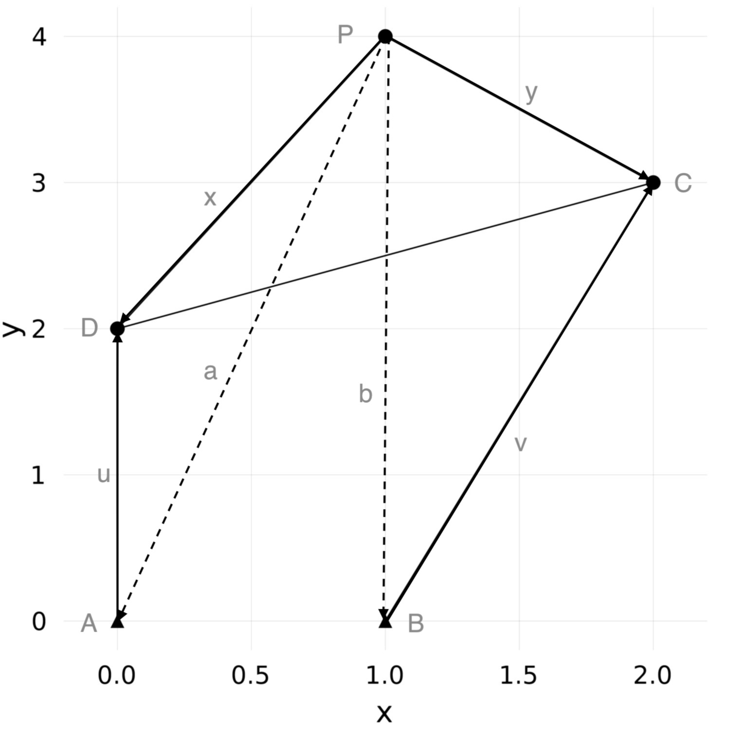
$A$ and $B$ are fixed hinges, $P$ denotes the coupler point. We have

$$ u = x-a \quad \text{and} \quad v = y-b.$$

Let $\lambda$ and $\mu$ denote the rotation of bars $u$ and $v$ and $\theta$ denotes the rotation of the coupler triangle $CPD$, as shown in the next picture.

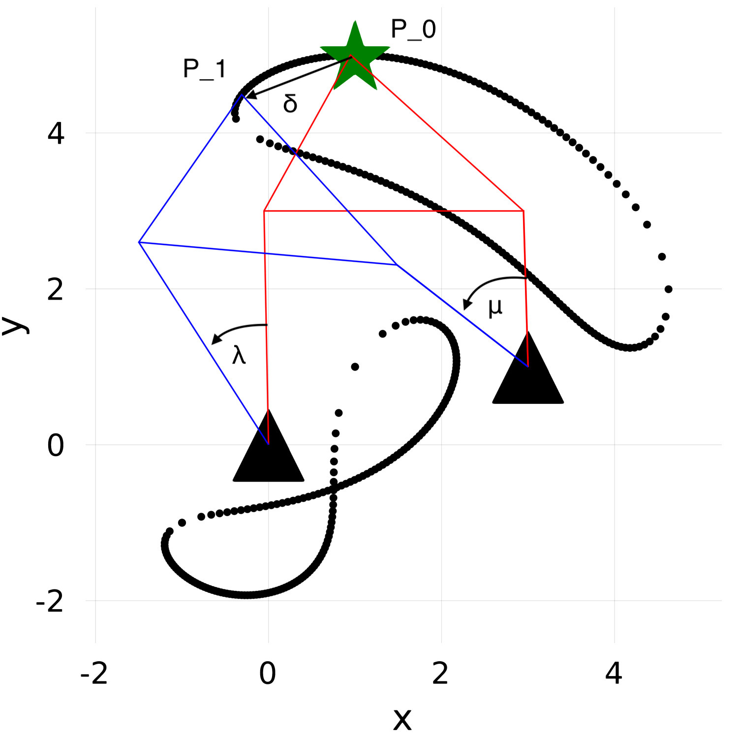
Here, $P_0$ and $P_1$ are two of the nine precision points. The black dots depict the associated coupler curve.

We have the following equations for $\lambda, \theta, \mu$:

$$ u e^{i \lambda_j} =x e^{i \theta_j} + P_j-P_0-a \quad \text{and}\quad y e^{i \mu_j} = y e^{i \theta_j} + P_j-P_0-b . $$

Setting $\delta_j = P_j-P_0$ for $j=1,\ldots,8$ we have

$$ (x-a) e^{i \lambda_j} =x e^{i \theta_j} + \delta_j -a \quad \text{and}\quad (y-b) e^{i \mu_j} = y e^{i \theta_j} + \delta_j -b $$

We need to make further reductions to get a polynomial system. Multiplying with the complex conjugates we have

$$ (x-a) e^{i \lambda_j} ( \overline{x}-\overline{a} ) e^{-i \lambda_j} = (x e^{i \theta_j} + \delta_j -a ) (\overline{x} e^{-i \theta_j} + \overline{\delta}_j -\overline{a}) $$

which is equivalent to

$$ \begin{array}{ll} &x\overline{x} -x\overline{a}-a\overline{x} +a\overline{a} \\ &= x\overline{x} + x \overline{\delta}_j e^{i \theta_j} -x\overline{a}e^{i \theta_j} +\delta_j \overline{x} e^{-i \theta_j} + \delta_j \overline{\delta}_j +\delta_j \overline{a} -a\overline{x} e^{-i \theta_j}-a\overline{\delta}_j +a\overline{a} \end{array} $$

A substitution of variables via $\gamma_i:= e^{i \theta_j}-1$ , finally gives us for $i\in \{1,\ldots ,8\}$

$$ (\overline a - \overline \delta_i)x\gamma_i+(a-\delta_i)\overline x \overline \gamma_i+(\overline a- \overline x)\delta_i+(a-x)\overline \delta_i-\delta_i\overline \delta_i =0 $$

Additionally, the $\gamma_i$ satisfy the following equality

$$ \gamma_i \overline \gamma_i+\gamma_i + \overline \gamma_i=0 $$

With a the same argument we also get

$$ (\overline b-\overline \delta_i)y\gamma_i+(b-\delta_i)\overline y\overline \gamma_i+(\overline b-\overline y)\delta_i+(b-y)\overline \delta_i-\delta_i\overline \delta_i =0. $$

The last three equations completely determine the coupler curve. However, they are not algebraic equations, because complex conjugation is not algebraic. To obtain a polynomial system we consider $x$ and $\bar{x}$ as independent variables (and similarly for all others). Afterwards, we filter out the solutions for which $x$ and $\bar{x}$ are not complex conjugates. We call the solutions where complex conjugation relations are satisfied real solutions since they correspond to real vectors in the plane.

Substituting the $\delta_i$s with our given precision points results in a polynomial system of $24$ variables in $24$ equations.

Solving the Nine Point Path Synthesis Problem

Similar to Wampler et. al. we first calculate all four bars for a given set of precision points and the track solutions to a new set of precision points. In order to calculate the start solution, we use monodromy to speed up the calculation.

This is the basic idea of the algorithm.

Take a random four bar and find $9$ random precision points on its coupler curve.
Given these $9$ precision points find all four bars whose coupler curve passes through them.
Given any $9$ new precision points find all fitting four bars tracking from the solution set of step $2$.
Filter all real solutions.

Step $1$ and $2$ need only be calculated once and can be used repeatedly to solve new problems.

First we define the variables in Julia.

using HomotopyContinuation

@polyvar x a y b x̄ ā ȳ b̄
@polyvar γ[1:8] γ̄[1:8]
@polyvar δ[1:8] δ̄[1:8]

Next we define the polynomial system as above.

#system of polynomials
D1 = [(ā * x - δ̄[i] * x) * γ[i] + (a * x̄ - δ[i] * x̄) *  γ̄[i] +
      (ā - x̄) * δ[i] + (a - x) * δ̄[i] - δ[i] * δ̄[i] for i in 1:8]
D2 = [(b̄ * y - δ̄[i] * y) * γ[i] + (b * ȳ - δ[i] * ȳ) * γ̄[i] +
      (b̄ - ȳ) * δ[i] + (b - y) * δ̄[i] - δ[i] * δ̄[i] for i in 1:8]
D3 = [γ[i] * γ̄[i] + γ[i] + γ̄[i] for i in 1:8]

fourbar_system = [D1; D2; D3]

Step 1

For our first step it is not necessary to pick a four bar with physical meaning. We generate $x, \overline{x}, a , \overline{a},…$ as random complex numbers. For $\gamma_1, …,\gamma_8, \overline{\gamma}_1,… \overline{\gamma}_8$ we generate random angles $\theta_1$,…,$\theta_8$ and then compute $\gamma_i:= e^{i \theta_j}-1$ and the conjugates respectively. Next we substitute these variables and solve D1 = D2 = 0 as equations in $\delta_1,\ldots,\delta_8$ and $\overline{\delta}_1,\ldots,\overline{\delta}_8$. This can be done separately for each $i\in {1,\ldots,8}$ as the pair of equations D1[i] = D2[i] = 0 only depends on $\delta_i$ and $\overline \delta_i$.

args = 2π * im .* rand(8)
Γ = exp.(args) .- 1
Γ̄ = exp.(-args) .- 1
xayb = randn(ComplexF64,8)

δδ̄_results = map(D1, D2) do d1, d2
    d = [d1; d2]
    start_sys = [subs(f, [x; a; y; b; x̄; ā; ȳ; b̄] => xayb, γ => Γ, γ̄ => Γ̄) for f in d]
    # only keep first solution
    first(solutions(solve(start_sys)))
end
δ_start = first.(δδ̄_results)
δ̄_start = last.(δδ̄_results)

Step 2

In the next step we turn our problem around. Instead of looking for the precision points we act as if we picked these precision points and wanted to find all other four bars whose coupler curves move through these precision points. Wampler et. al. showed that there are $6 \cdot 1442 = 8652$ solutions for this polynomial system.

Since we already have one solution we can use monodromy to find all other solutions. In order to speed up the calculation we can exploit two group actions acting on the solution set.

Group Actions

One group action appears when we relabel the bars. If we exchange $x$ and $y$, $a$ and $b$ etc. we also get a valid solution. This group action halves the number of solutions leaving us with 4326 solutions modulo this group action.

# Switch roles of (x,a) and (y,b).
# We have the variable ordering x a y b x̂ â ŷ b̂
# so we need to switch to y b x a ŷ b̂ x̂ â
relabeling(s) = [[s[3],s[4],s[1],s[2],s[7],s[8],s[5],s[6]]; s[9:24]]

The next group action is due to Roberts. It states that given a four bar, we can find two related four bars (called Roberts cognates) that follow the same coupler curve: $$ r(x,a,y,b,\theta, \lambda, \mu) = \left(\frac{(x-a)y}{x-y}, \frac{bx-ay}{x-y},a-x,a, \lambda, \mu, \theta\right). $$ These cognates are also solutions of our problem. This leaves us with $1442$ solutions modulo both group actions.

Since $\theta, \lambda, \mu$ aren't variables of our system, we make the following adjustment: substitute $x,a,y,b$ and $\theta=\gamma_i+1$ and define $\lambda$ and $\mu$ as follows

$$ \lambda_j = \frac{x \theta_j + \delta_j -a}{x-a } \quad \text{and} \quad \mu_j = \frac{y \theta_j + \delta_j -b}{y-b}. $$

Since the Roberts’ cognates depend on $\delta_j$ and $\bar{\delta}_j$ we have to give the values of Γ and Γ̄ to the implementation in the FourBarLinkages package

roberts_cognates(s) = FourBarLinkages.roberts_cognates(s, δ_start, δ̄_start)

Computing all solutions

Here is the code for computing all solutions with monodromy.

start_solution = [xayb; Γ; Γ̄]
start_params  = [δ_start; δ̄_start]

monodromy_result = monodromy_solve(fourbar_system, start_solution, start_params;
                                   parameters = [δ; δ̄],
                                   group_actions = [relabeling, roberts_cognates],
                                   target_solutions_count = 1442)

start_solutions = solutions(monodromy_result)

Step 3

For the third step we track from our set of start solutions to any solution given nine precision points. Assume we are given the 9 coupler_points from the beginning. For them this looks as follows:

δ = coupler_points[2:9] .- coupler_points[1]
δ̄ = conj.(δ)
final_result = solve(fourbar_system, start_solutions;
                     parameters = [δ; δ̄],
                     start_parameters = start_params,
                     target_parameters=[δ; δ̄])

results = solutions(final_result)

Step 4

Since we are only interested in solutions with physical meaning, we now filter for real solutions. This we can do by checking if $\mathrm{conj}(x) \approx \overline{x}$, $\mathrm{conj}(y) \approx \overline{y}$,…

real_fourbars = filter(s -> all(i -> s[i] ≈ conj(s[i+4]), 1:4), solutions(final_result))

Results

Following Wampler et al. we try our method on the following examples:

random example

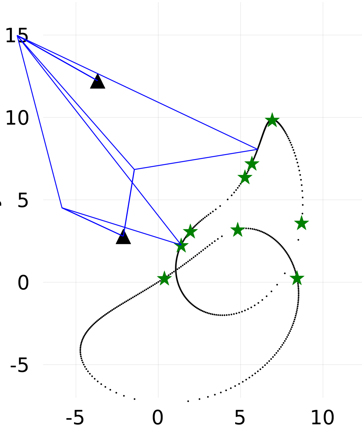
all points are positioned on an oval

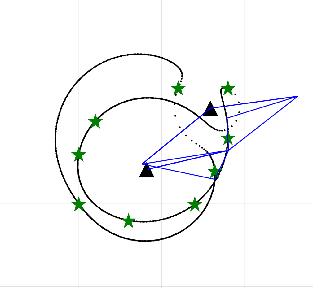
3 points on one circle, 4 on another

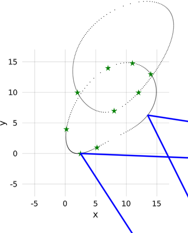
5 points on a line, 4 on another

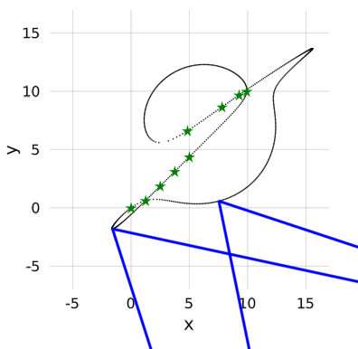
In the pictures one can see that the coupler curve is not necessarily connected.

Cite this example:

@Misc{ alts-problem2023 ,
    author =  { Paul Breiding, Anna Eckhardt and Sascha Timme },
    title = { Alt's problem },
    howpublished = { \url{ https://www.JuliaHomotopyContinuation.org/examples/alts-problem/ } },
    note = { Accessed: March 10, 2023 }
}

Published by Paul Breiding, Anna Eckhardt and Sascha Timme 28 Oct, 2019