The following example is from Section 7.3 in A. Sommese, C. Wampler: The Numerical Solution of Systems of Polynomial Arising in Engineering and Science
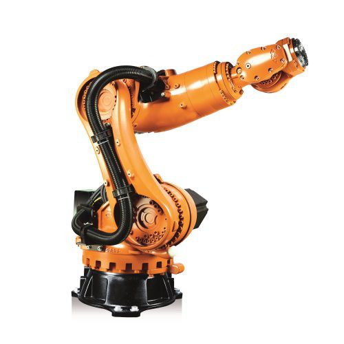
Consider a robot that consists of 7 links connected by 6 joints. The first link is fixed on the ground and the last link has a “hand”. The problem of determining the position of the hand when knowing the arrangement of the joints is called forward problem. The problem of determining any arrangement of joints that realized a fixed position of the hand is called backward problem.
- $z_i \cdot z_i = 1, i=1,\ldots,6.$
- $z_1 \cdot z_2 = \cos \alpha_1,\ldots, z_5 \cdot z_6 = \cos \alpha_5$.
- $a_1 (z_1 \times z_2) + \cdots + a_5 (z_5 \times z_6) + a_6 z_2 + \cdots + a_9 z_5= p.$
for $\alpha=(\alpha_1\ldots, \alpha_5)$ and $a=(a_1,\ldots,a_9)$ and $p=(p_1,p_2,p_3)$. The $\alpha_i$ are the “twist angle” between joints, the $a_i$ are the “link length” between joint axes and the $p$ encodes the position of the hand. Here $\times$ is the cross product in $\mathbb{R}^3$.
see the above reference for a detailed explanation on how these numbers are to be interpreted). Here $\times$ is the cross product in $\mathbb{R}^3$.
In this notation the forward problem consists of computing $(\alpha,a)$ given the $z_i$ and $p$ and the backward problem consists of computing $z_2,\ldots,z_5$ that realize some fixed $(\alpha,a,p,z_1,z_6)$ (knowing $z_1,z_6$ means that the position where the robot is attached to the ground and the position where its hand should be are fixed).
Assume that $z_1$ and $z_6$ are random unit vectors, $p=(1,1,0)$ and some random $a$ and $\alpha$. We compute all backward solutions. We start with setting up the system.
using HomotopyContinuation, LinearAlgebra
# initialize the variables
@var z[1:6,1:3] p[1:3]
α = randn(5)
a = randn(9)
# define the system of polynomials
f = [z[i,:] ⋅ z[i,:] for i = 2:5]
g = [z[i,:] ⋅ z[i+1,:] for i = 1:5]
h = sum(a[i] .* (z[i,:] × z[i+1,:]) for i=1:3) +
    sum(a[i+4] .* z[i,:] for i = 2:5)
F′ = [f .- 1; g .- cos.(α); h .- p]
# assign values to z₁ and z₆
z₁ = normalize!(randn(3))
z₆ = normalize!(randn(3))
F = [subs(f, z[1,:]=>z₁, z[6,:]=>z₆, p=>[1, 1, 0]) for f in F′]
Now we can just pass F to solve in order to compute all solutions.
julia> solve(F; start_system = :total_degree)
Result with 16 solutions
========================
• 1024 paths tracked
• 16 non-singular solutions (0 real)
• random_seed: 0xb809e6ce
• start_system: :total_degree
We find 16 solutions, which is the correct number of solutions for these type of systems.
But if we study the problem a little bit closer, we can see that the equations are bi-homogeneous with respect to the variable groups $\{z_2, z_4\}$ and $\{z_3, z_5\}$. The multi-homogeneous Bezout number with respect ot this variable group is
variable_groups = [[z[2,:]; z[4,:]], [z[3,:]; z[5,:]]]
paths_to_track(System(F; variable_groups=variable_groups); start_system = :total_degree)
320
We can use this to solve the system more efficiently
julia> solve(F; variable_groups=variable_groups, start_system = :total_degree)
Result with 16 solutions
==================================
• 16 non-singular solutions (0 real)
• 0 singular solutions (0 real)
• 320 paths tracked
• random seed: 923247
Solving the inverse problem repeatedly
Now assume that we do not only want to know solve the inverse problem for one value of p but rather for many different positions of the hand.
Instead of solving the system from scratch every time (and tracking 324 paths) we can first compute as set of 16 solutions with respect to a “generic” (complex) set of parameters (offline phase) and then use these start solutions to compute the solutions for the specific parameters we are interested in (online phase). We can do this by using a parameter homotopy.
Let's start with computing a generic instance.
p_rand = randn(ComplexF64, 3)
F̂ = System([subs(f, z[1,:]=>z₁, z[6,:]=>z₆) for f in F′], parameters = p,  variable_groups=variable_groups)
R_rand = solve(F̂, target_parameters = p_rand, start_system = :total_degree)
Result with 16 solutions
========================
• 320 paths tracked
• 16 non-singular solutions (0 real)
• random_seed: 0xf04f1c49
• start_system: :total_degree
Now we can use this to solve for our specific value $q=[2,3,4]$:
q = [2,3,4]
solve(F̂, solutions(R_rand); start_parameters=p_rand, target_parameters=q)
Result with 16 solutions
==================================
• 16 non-singular solutions (0 real)
• 0 singular solutions (0 real)
• 16 paths tracked
• random seed: 231232
And we obtain 16 new solutions, but this time we only needed to track 16 paths. For even more performance improvements you can take a look at our guide regarding the solution of many systems in a loop.
Cite this example:
@Misc{ 6Rlinkrobot2026 ,
    author =  { Sascha Timme },
    title = { The 6R-serial link robot },
    howpublished = { \url{ https://www.JuliaHomotopyContinuation.org/examples/6rlinkrobot/ } },
    note = { Accessed: February 5, 2026 }
}